Simulating Distributions & Variables In R

Introduction (PDF & R-Code)

Consistent with the goals of the series, we will discuss how to specify data simulations satisfying the assumptions – rules – that we want to exist within the data. Nevertheless, before we being defining relationships and constructing dataframes, we must learn how to specify a vector of values (e.g, a variable) from the distributions at our disposal within the base R package. Our discussions will review the specifications for drawing values from various distributions, as opposed to discussing the property of the distributions. Please feel free to edit the code provided to see how different specifications alter the distributional properties of the created vectors

Specifying a Vector (Variable)

In R, vectors can be created by saving a series of numbers with a label (X is the label in the code below). To save information to a label you can use an <- or an =, but personally I am more inclined to use the <-. In the code below, we save a vector of 100 rows with increasing numbers – 1, 2, 3, 4, …, 100 – using the c() as X.  Moreover, we save 1 row with the value of 3.2 as V.

X<-c(1:100)
V<-3.2

Distributions

Drawing random numbers from distributions is fundamental to simulating data for three reasons: (1) there is no unknown bias in the manner in which numbers are drawn, (2) the process can be replicated with the set.seed function, and (3) we know the distributional assumptions underlying the specified variable. While the specification for drawing values from every distribution available in base R is reviewed below, our data simulations will primarily employ the uniform distribution, normal distribution, binomial distribution, negative binomial distribution, Poisson distribution, and an exponential distribution. Nevertheless, when we encounter the need to specify alternative distributions, we will reference this entry or combined distributional specifications.

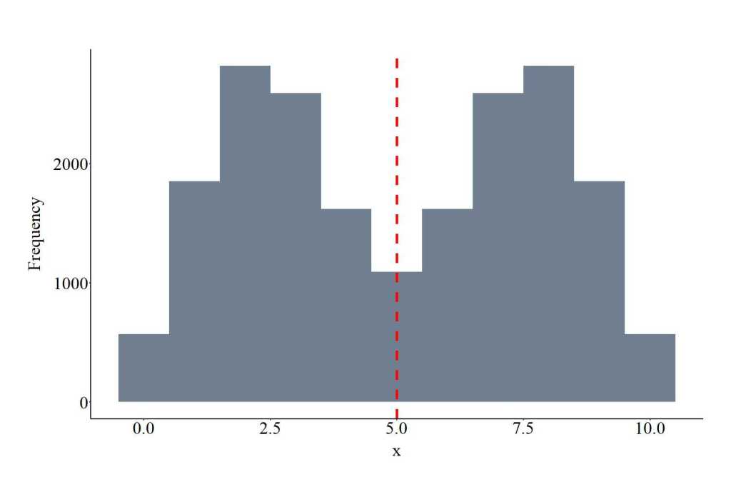
Drawing Values From a Uniform Distribution

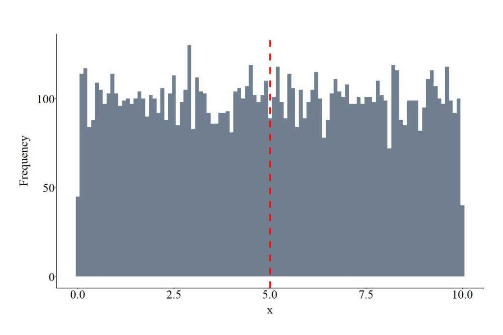
Alongside the normal distribution, we will commonly draw values from uniform distribution. The function runif requires users to specify the number of draws (10000 in the code), the minimum and maximum values of the distribution (0 and 10, respectively). The minimum and maximum values serve as a threshold where values less than 0 or greater than 10 have no likelihood of being selected, but every value in between has an equal likelihood of being selected. Min and max can be any value. The plot below shows the values drawn from the uniform distribution using the specification below.

UD<-runif(10000, min = 0, max = 10)

Drawing Values From a Normal Distribution

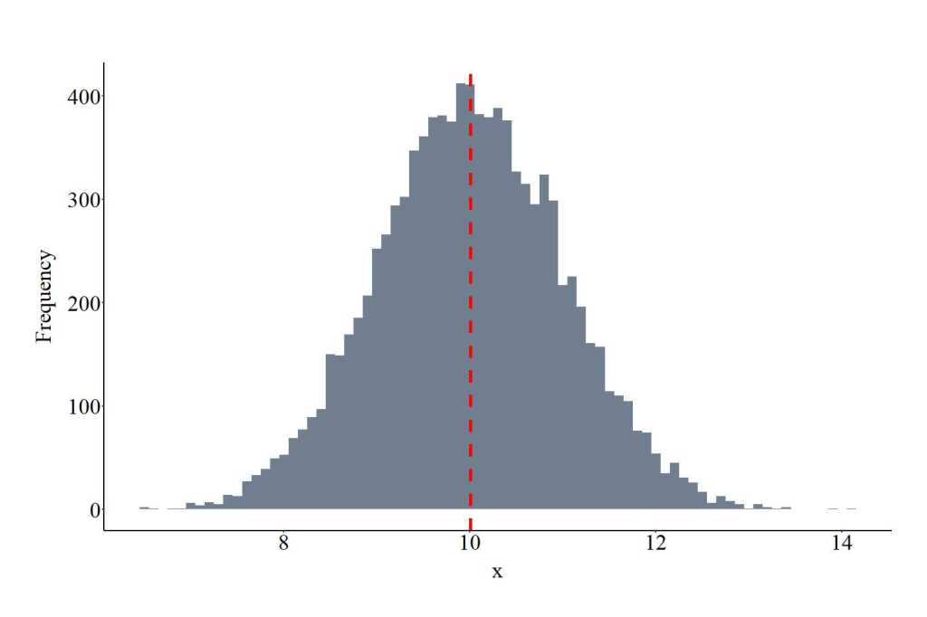
The function rnorm provides the ability to draw values from a normal distribution – or Gaussian distribution. The function requires users to specify the number of draws (10000 in the code), the mean and standard deviation of the distribution (10 and 1, respectively). Mean can be any value, while sd must be greater than 0. The plot below shows the values drawn from the normal distribution using the specification below.

GD<-rnorm(10000 ,mean = 10, sd = 1)

Drawing Values From a Binomial Distribution

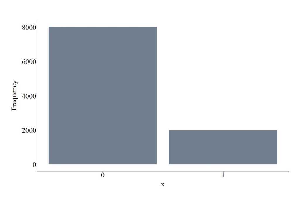
The function rbinom provides the ability to draw values from a binomial distribution – or Benoulli distribution. The function requires users to specify the number of draws (10000 in the code), the size and the probability of the distribution (1 and .20, respectively). The size represents the number of trials (if size is > 1 a discrete variable can be generated with as many trials), while the prob provides an indication of how likely selection is (0,1) for each trial. Size must be a positive integer and prob must be > 0 and <= 1. The plot below shows the values drawn from the binomial distribution using the specification below. Importantly, only integers – whole numbers – will be drawn from the distribution.

BID<-rbinom(10000, size = 1, prob=.20)

Drawing Values From a Negative Binomial Distribution

The function rnbinom provides the ability to draw values from a negative binomial distribution. As a reminder, negative binomial distribution is often over dispersed. The function requires users to specify the number of draws (10000 in the code), the size and the probability of the distribution (1 and .20, respectively). Distinct from the binomial specification, size represents the desired number of successful trials (or dispersion parameter), while the prob provides an indication of how likely selection is (0,1) for each trial. Size must be positive integer and prob must be > 0 and <= 1. The plot below shows the values drawn from the negative binomial distribution using the specification below. Only integers will be drawn from the distribution.

NBID<-rnbinom(10000, size = 1, prob = .50)

Drawing Values From a Poisson Distribution

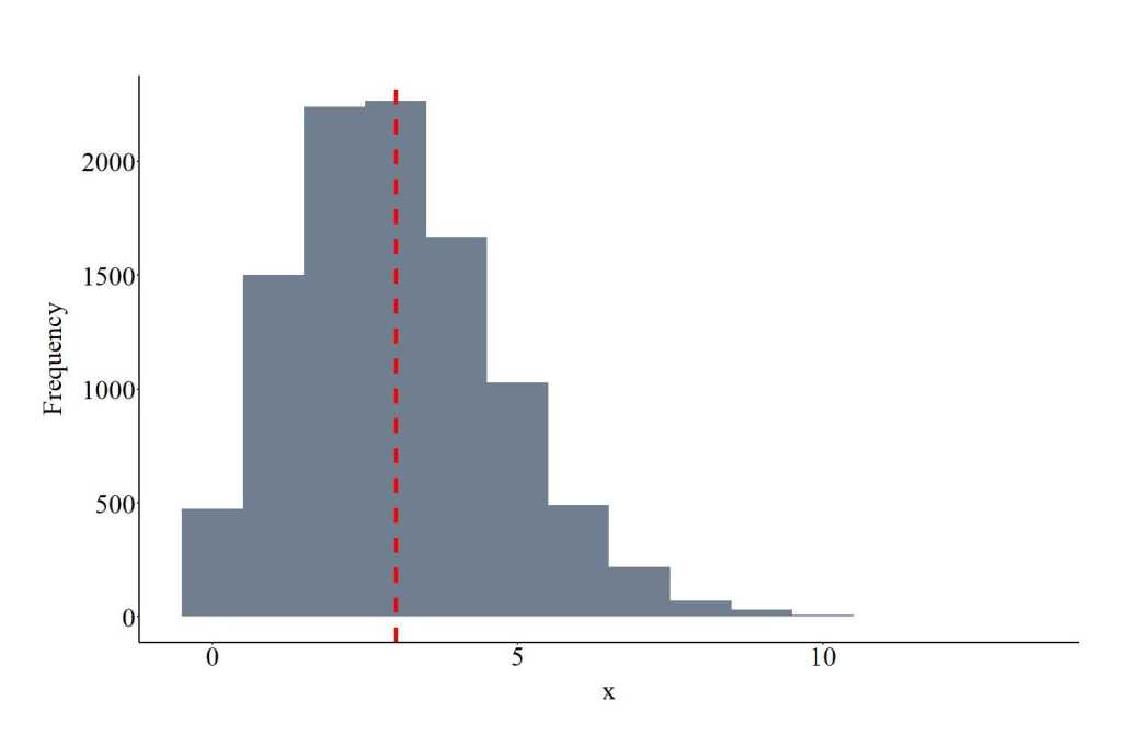
The function rpois provides the ability to draw values from a Poisson distribution. The function requires users to specify the number of draws (10000 in the code), the lambda value. The lambda value represents the mean of the distribution and must be positive. The plot below shows the values drawn from the Poisson distribution using the specification below. Only integers will be drawn from the distribution.

POID<-rpois(10000, lambda = 3)

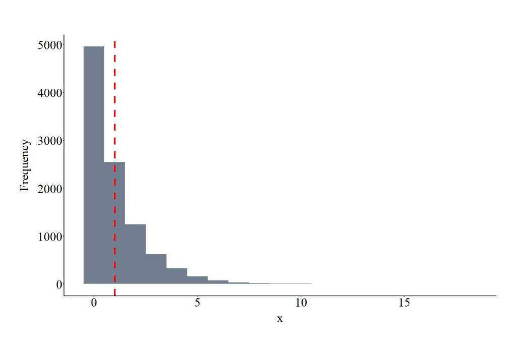
Drawing Values From an Exponential Distribution

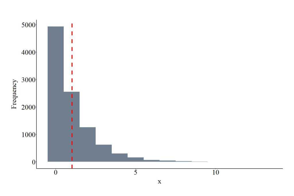
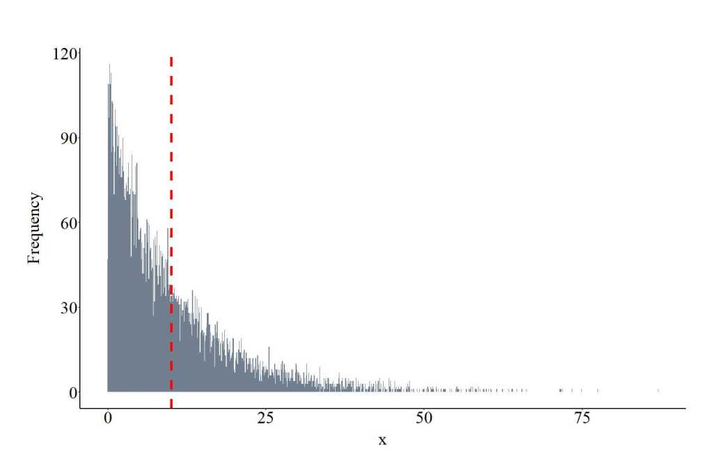
The function rexp provides the ability to draw values from an exponential distribution. The function requires users to specify the number of draws (10000 in the code), the rate for the exponential distribution. The rate represents the rate of the density across the distribution. The rate is required to be a positive value. The plot below shows the values drawn from the exponential distribution using the specification below.

EXD<-rexp(10000, rate = .10)

Drawing Values From a Beta Distribution

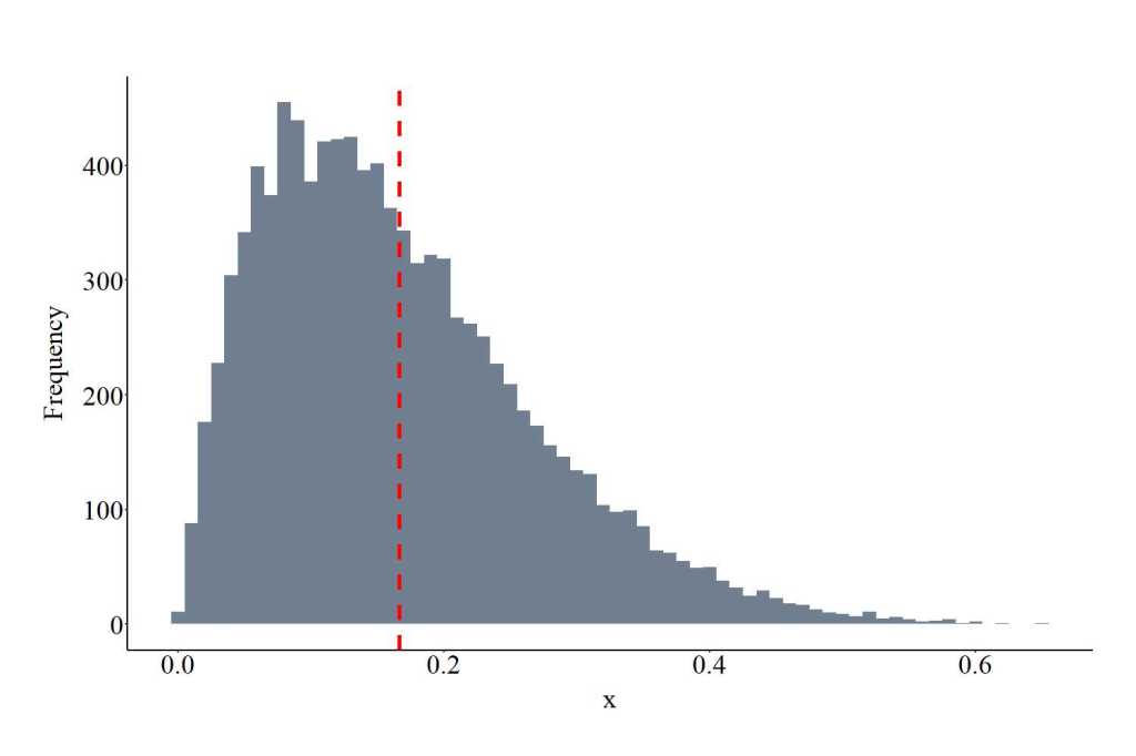
The function rbeta provides the ability to draw values from a beta distribution. The function requires users to specify the number of draws (10000 in the code), shape1, shape 2, and ncp. shape1 and shape2 represent the parameters for the beta distribution, while ncp represents the non-centrality parameter. All of the required specifications must be positive integers. The plot below shows the values drawn from the beta distribution using the specification below. Importantly, only values between 0 and 1 will be drawn from the distribution.

BED<-rbeta(10000, shape1 = 2, shape2 = 10, ncp = 0)

Drawing Values From a Cauchy Distribution

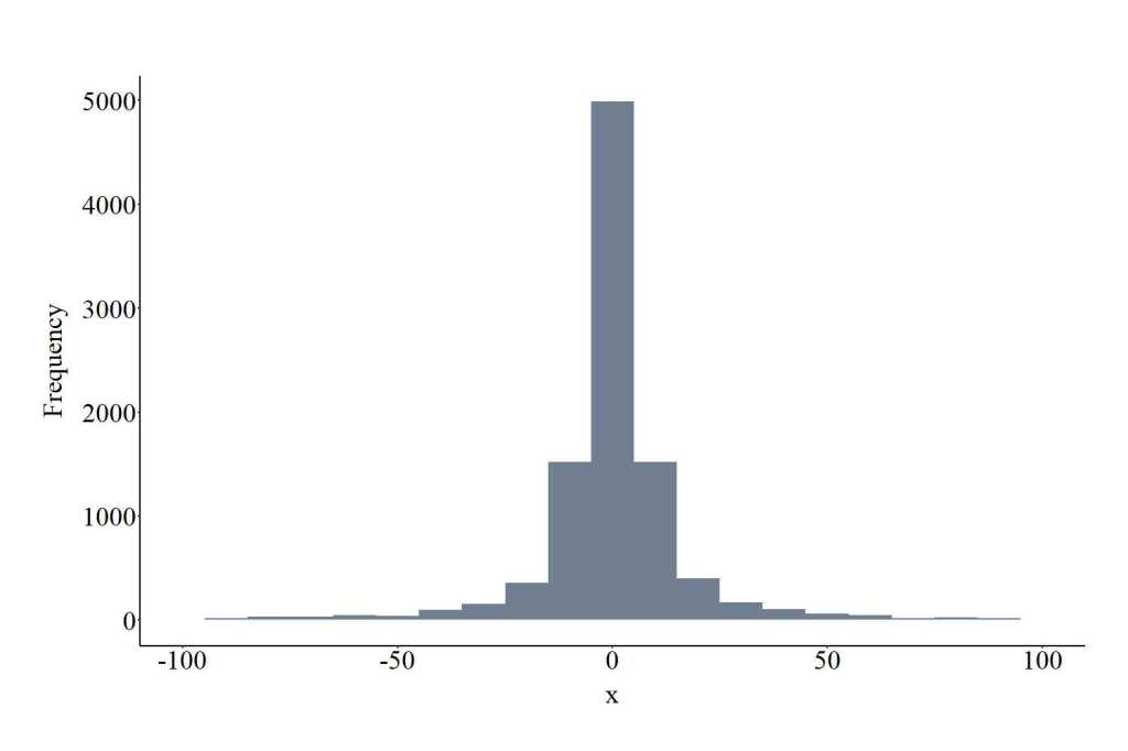
The function rcauchy provides the ability to draw values from a Cauchy distribution. The function requires users to specify the number of draws (10000 in the code), the location and the scale of the distribution. The location represents the peak of the distribution, while the scale represents the density of the distribution (larger values wider density). Scale must be specified with positive integers. The plot below shows the values drawn from the Cauchy distribution using the specification below.

CAD<-rcauchy(10000, location = 0, scale= 5)

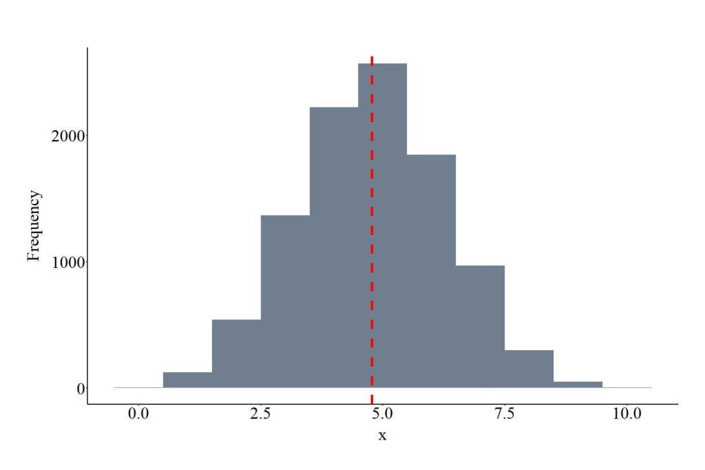
Drawing Values From a F Distribution

The function rf provides the ability to draw values from a F distribution. The function requires users to specify the number of draws (10000 in the code), df1, df2, and ncp. df1 and df2 represent the degrees of freedom for the distribution, while ncp represents the non-centrality parameter. df1, df2, and ncp must be specified with positive integers. The plot below shows the values drawn from the F distribution using the specification below.

FD<-rf(10000, df1 = 10, df2 = 10, ncp = 10)

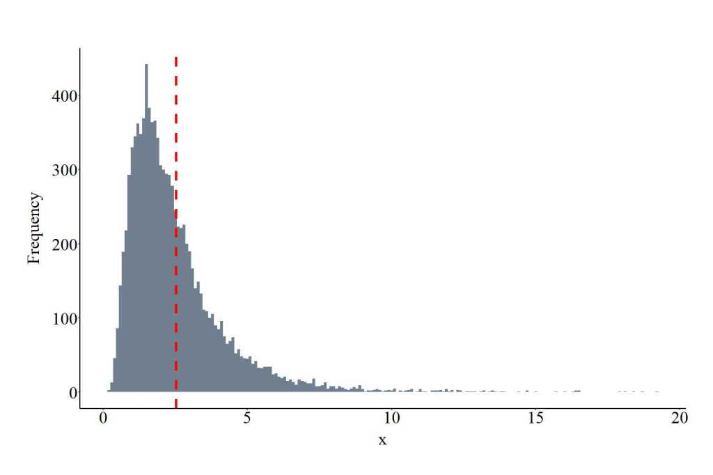
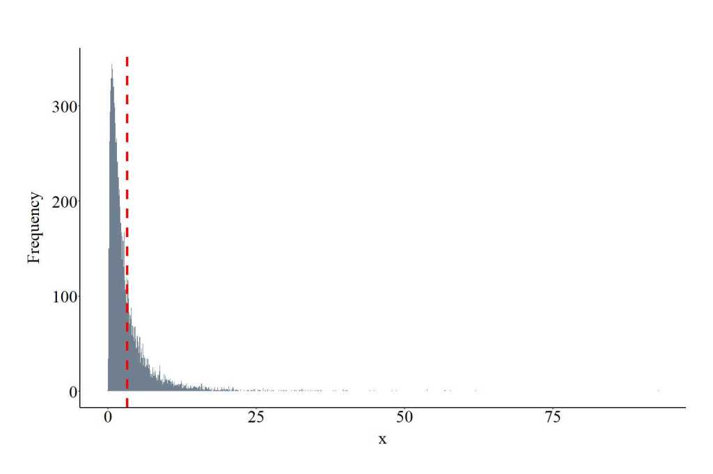
Drawing Values From a Gamma Distribution

The function rgamma provides the ability to draw values from a gamma distribution. The function requires users to specify the number of draws (10000 in the code), shape and rate. Shape represents the spread of the distribution, while rate represents the rate of the density across the distribution. Both shape and rate are required to be positive values, where smaller values for shape center the distribution on 0, while smaller values for rate extend the range of the distribution. The plot below shows the values drawn from the gamma distribution using the specification below.

GAD<-rgamma(10000, shape = 2, rate = 1)

Drawing Values From a Geometric (Negative Binomial) Distribution

The function rgoem provides the ability to draw values from a geometric negative binomial distribution. The function requires users to specify the number of draws (10000 in the code) and the probability of the distribution (.50). prob provides an indication of how likely selection is (0,1) for each trial. prob must be > 0 and <= 1. The plot below shows the values drawn from the geometric negative binomial distribution using the specification below. Only integers will be drawn from the distribution.

GEOD<-rgeom(10000, prob = .50)

Drawing Values From a Hyper-Geometric Distribution

The function rhyper provides the ability to draw values from a hyper-geometric negative binomial distribution. The function requires users to specify the number of draws (10000 in the code), m, n, and k. m represents the number of white balls in an urn, n represents the number of black balls, and k represents the number of balls drawn from the earn. m, n, and k must be positive integers. The plot below shows the values drawn from the hyper-geometric negative binomial distribution using the specification below. Only integers will be drawn from the distribution.

RHYD<-rhyper(10000, m = 10, n = 200, k = 100)

Drawing Values From a Log Normal Distribution

The function rlnorm provides the ability to draw values from a log normal distribution. The function requires users to specify the number of draws (10000 in the code), meanlog of the log distribution (specified as log[2]) and the sdlog. meanlog and sdlog are required to be positive values. The plot below shows the values drawn from the log normal distribution using the specification below.

LNOD<-rlnorm(10000, meanlog = log(2), sdlog = 1)

Drawing Values From a Multinomial Distribution

The function rmultinom provides the ability to draw values from a multinomial distribution. The function requires users to specify the number of draws (10000 in the code), the size and the probability of the distribution. The size represents the number of trials (if size is > 1 a discrete variable can be generated with as many trials), while the prob provides an indication of how likely selection is (0,1) for each trial. Importantly, for a multinomial distribution 2 or more probabilities are required to be specified using c(). Size must be a positive integer and prob must be > 0 and <= 1. The plot below shows the values drawn from the binomial distribution using the specification below. Importantly, only integers – whole numbers – will be drawn from the distribution.

MNOD<-rmultinom(10000, size = 10, prob = c(0.1,.3))

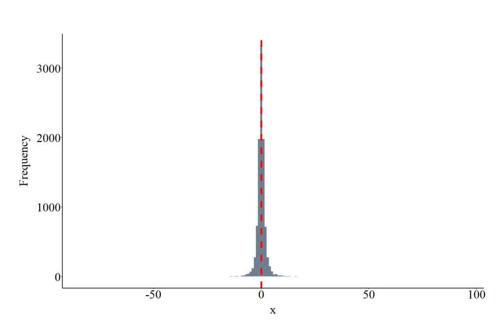
Drawing Values From a Student’s T Distribution

The function rt provides the ability to draw values from a t distribution. The function requires users to specify the number of draws (10000 in the code) and df. df represents the degrees of freedom, which is required to be a positive integer. Higher degrees of freedom generates a narrower distribution. The plot below shows the values drawn from the t distribution using the specification below.

TD<-rt(10000, df = 2)

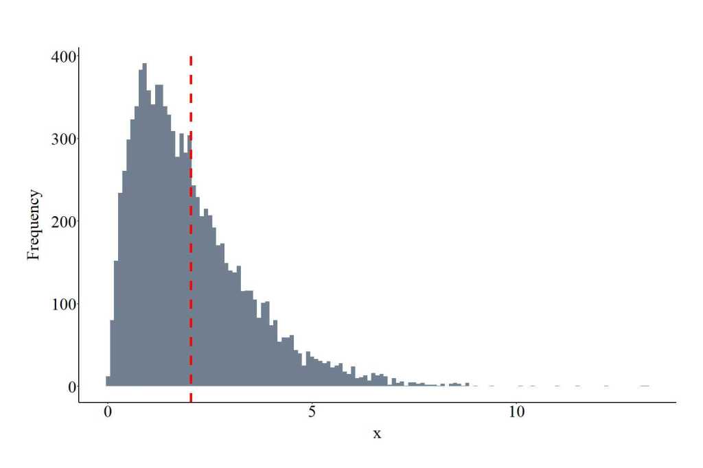
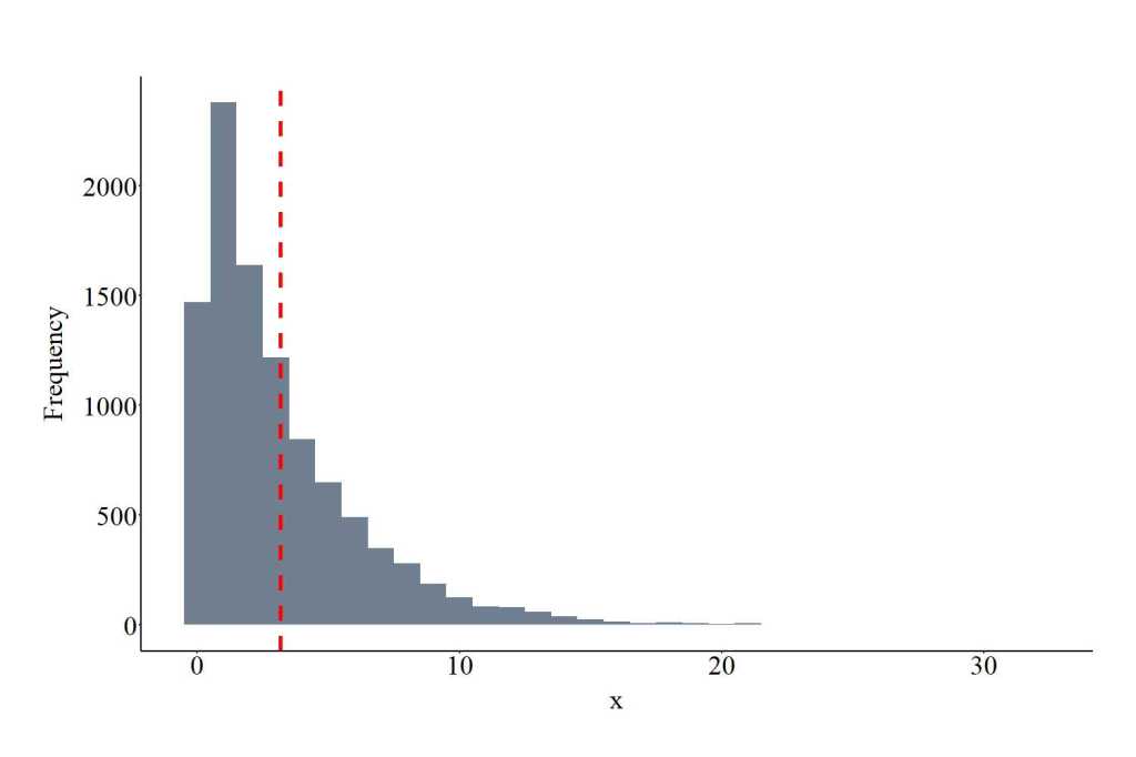
Drawing Values From a Weibull Distribution

The function rweibull provides the ability to draw values from a Weibull distribution. The function requires users to specify the number of draws (10000 in the code), the shape, and scale. Shape represents the spread of the distribution, while the scale represents the density of the distribution (larger values wider density). Both shape and scale are required to be positive values, where smaller values of shape widen the distribution, while smaller values for scale narrow the distribution tail. The plot below shows the values drawn from the Weibull distribution using the specification below.

WEID<-rweibull(10000, shape = 1, scale = pi)

License: Creative Commons Attribution 4.0 International (CC By 4.0)