I apologize; In previous entry I used the term balance to refer to the similarities between the treatment and control group on the key covariates before and after the matching procedure was conducted. By rule of thumb, balance is used to describe the similarities between the treatment and control groups after matching, while common supportis used to describe the similarities between the treatment and control groups before matching. The difference of terms directly relates to a fundamental assumption of quasi-experimental matching techniques: The Assumption of Common Support.
Quasi-experimental matching techniques are designed to match treatment to similar control participants to approximate the counterfactual condition created when a true experiment is conducted. Although the process of matching can vary drastically, every procedure requires the treatment and control cases to be similar enough to match. The more similar the treatment and control cases are, the easier it is to match. If the treatment and control groups have no overlapping characteristics, however, a counterfactual condition cannot be generated through matching. This is the assumption of common support. Explicitly, we assume that enough distributional overlap exists between the treatment and control groups to permit the matching of participants. Within the context of propensity score matching, the assumption of common support requires users to have a large amount of distributional overlap between the treatment and control groups on all of the matching constructs as well as the predicted probabilities. When weak or no common support exists between the treatment and control groups, we have violated the assumption of common support and will produce biased post-matching estimates (if we even have any appropriate matches).
Demonstrating Common Support
Let’s start by simulating our data. For simplicity, we are only going to specify two normally distributed independent variables: SCV1 & CV1. After simulating the independent variables, we can set the continuous treatment variable to be equal to .30*SCV1, .0001*CV1, and 2.0* a normal distribution with a mean of zero and a standard deviation of 2.5. Succeeding the specification of the continuous treatment variable, we can create the dichotomized treatment variable. This can be achieved by splitting the continuous treatment variable at the mean, where any case with a score greater than 13.75 will be exposed to the treatment (receive a “1” on TDI) and any case with a score less than or equal to 13.75 will not be exposed to the treatment (receive a “0” on TDI). After simulating TDI, we can specify the dependent variable (Y). Y was specified to equal .50 *TDI, .01*SCVI, and .01*CV1. Finally, we can check our simulations by running two regression models: (1) Y regressed on TDI and (2) Y regressed on TDI, SCV1, and CV1. Consistent with the specifications, the estimated relationship between Y and TDI in the first regression model is upwardly biased (because of the confounding influence of SCV1 and CV1), while the second regression model provides the true estimate (.50).
> ### Simulating Data ####
> N<-1000
> set.seed(23733)
> SCV1<-trunc(rnorm(N,35,5)) # Semi-continuous Variable
> set.seed(29204)
> CV1<-trunc(rnorm(N,35000,5000)) # Continuous Variable
>
> Data<-data.frame(SCV1,CV1)
>
>
> ### Creating Continuous Treatment Variable ####
>
> set.seed(1992)
> Data$TCon<-.30*Data$SCV1+.0001*Data$CV1+2.0*rnorm(N,0,10)
>
>
> summary(Data$TCon)
   Min. 1st Qu.  Median    Mean 3rd Qu.    Max.
 -47.56    0.75   13.71   13.75   26.95   77.09
>
>
> ### Creating Dichotomous Treatment Variable ####
>
> mean(Data$TCon)
[1] 13.75
>
> table(Data$TCon>13.75)

FALSE  TRUE
  501   499
> Data$TDI[Data$TCon>13.75]<-1
> Data$TDI[Data$TCon<=13.75]<-0
> table(Data$TDI)

  0   1
501 499
>
>
>
>
> ### Creating Dependent Variable ####
>
>
> Data$Y<-.50*Data$TDI+.01*Data$SCV1+.01*Data$CV1
>
>
>
> ### Checking Simulations ####
>
> lm(Y~TDI, data = Data)

Call:
lm(formula = Y ~ TDI, data = Data)

Coefficients:
(Intercept)          TDI
      348.5          5.4

> lm(Y~TDI+SCV1+CV1, data = Data)

Call:
lm(formula = Y ~ TDI + SCV1 + CV1, data = Data)

Coefficients:
      (Intercept)                TDI               SCV1                CV1
0.000000000000492  0.500000000000025  0.010000000000002  0.010000000000000
Now let’s explore the common support between the treatment and control cases on SCV1 and CV1. Panel A illustrates the common support for SCV1, while Panel B illustrates the common support for SCV1. The gray area in the figures below represents the treatment cases, the light red area represents the control cases, and the dark red represents the distributional overlap between the treatment and control groups. As it can be observed, a large amount of support (i.e., distributional overlap) exists between the treatment and control groups on both SCV1 and CV1, which suggests that we have satisfied the assumption of common support.
Panel A
Panel B
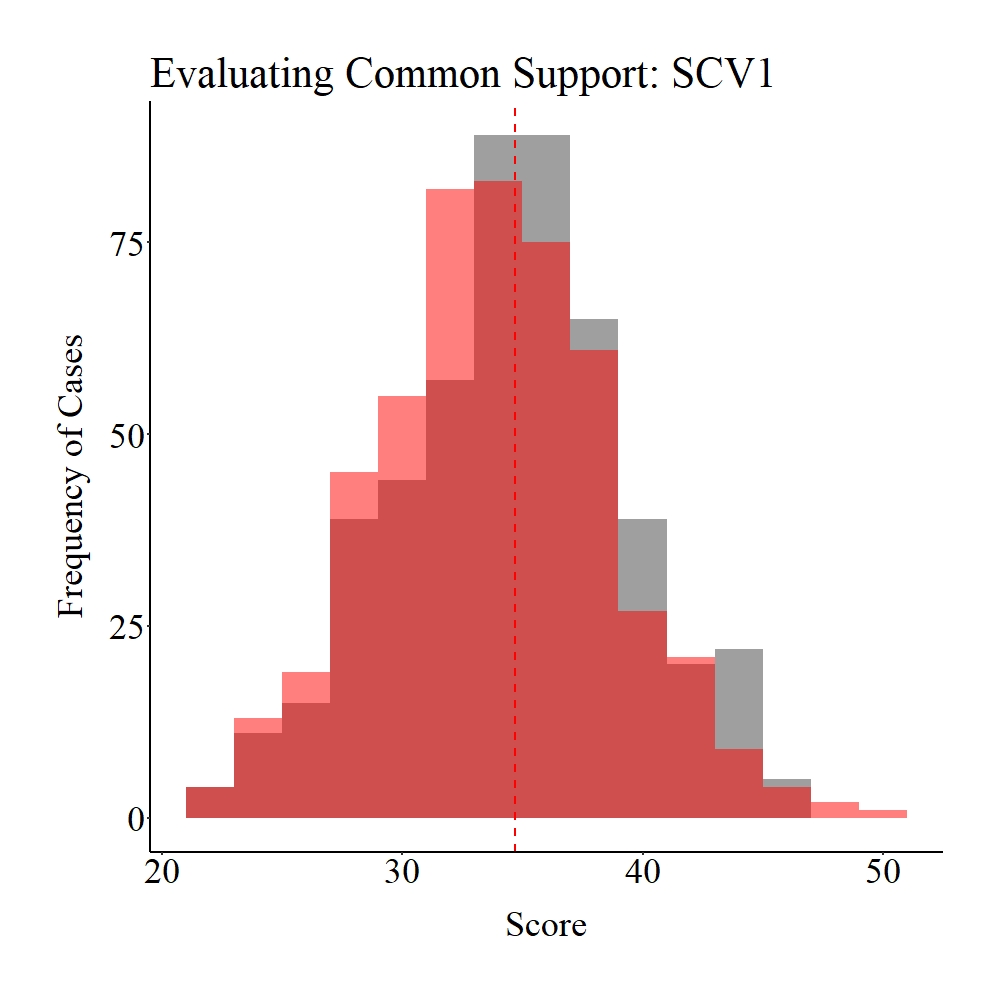
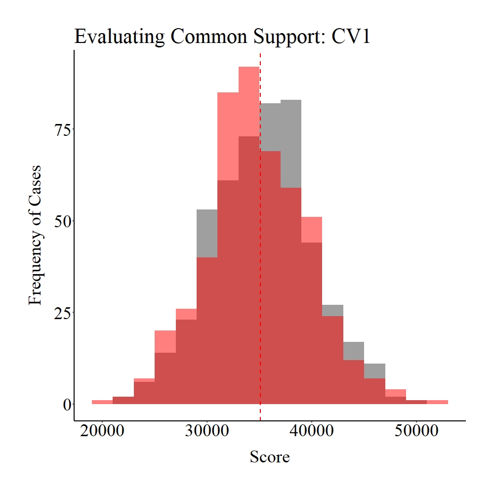
Figure Notes: The gray area represents the treatment cases only, the light red area represents the control cases only, and the dark red represents the overlap between the groups.
Consistent with satisfying the assumption of common support, we can conduct a matching procedure with this sample. For simplicity, we matched the treatment to control cases using 1-1 nearest neighbor matching with a random order, without replacement, and with a caliper of .05. This matching procedure resulted in the creation of a matched subsample containing 854 cases (427 treatment and 427 control cases).
> ### Matching (Nearest Neighbor, Random, 1 to 1) one time all variables ####
>
> set.seed(1992)
> M1<-matchit(TDI~SCV1+CV1, data = Data,
+             method = "nearest", m.order = "random", ratio = 1, replace = FALSE, caliper = .05)
>
> summary(M1)

Call:
matchit(formula = TDI ~ SCV1 + CV1, data = Data, method = "nearest",
    replace = FALSE, m.order = "random", caliper = 0.05, ratio = 1)

Summary of Balance for All Data:
         Means Treated Means Control Std. Mean Diff. Var. Ratio eCDF Mean eCDF Max
distance         0.503         0.495           0.183      0.985     0.054    0.101
SCV1            35.058        34.323           0.151      1.019     0.026    0.094
CV1          35306.892     34817.557           0.101      0.967     0.032    0.096


Summary of Balance for Matched Data:
         Means Treated Means Control Std. Mean Diff. Var. Ratio eCDF Mean eCDF Max
distance           0.5          0.50          -0.000      0.998     0.003    0.014
SCV1              34.8         34.67           0.026      0.968     0.008    0.052
CV1            35103.0      35297.69          -0.040      1.022     0.018    0.054
         Std. Pair Dist.
distance           0.010
SCV1               0.650
CV1                1.004

Percent Balance Improvement:
         Std. Mean Diff. Var. Ratio eCDF Mean eCDF Max
distance            99.9       84.7      95.1     86.0
SCV1                82.8      -67.9      70.4     45.4
CV1                 60.2       35.0      43.0     43.8

Sample Sizes:
          Control Treated
All           501     499
Matched       427     427
Unmatched      74      72
Discarded       0       0

>
> M1DF<-match.data(M1)
>
Succeeding the matching procedure, we can evaluate the balance (we switched the terms because we are talking about post-matching evaluations) in the matched data. Unlike Entry 6, we will rely on visualizations to quickly evaluate the balance created by the matching procedure.[i] As demonstrated below – and supported by the results in the code above – the matching procedure increased (slightly) the balance between the treatment and control groups.
Panel A
Panel B
Panel C
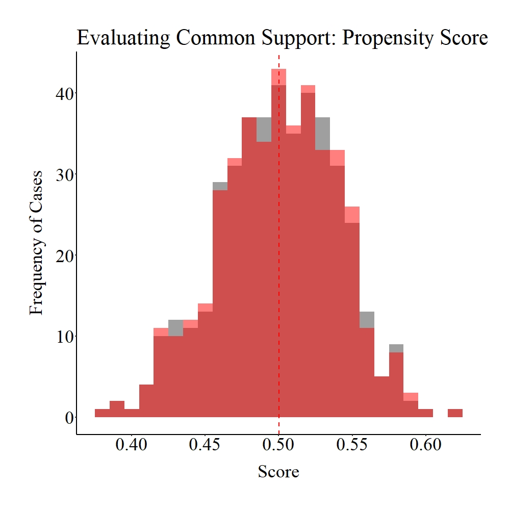
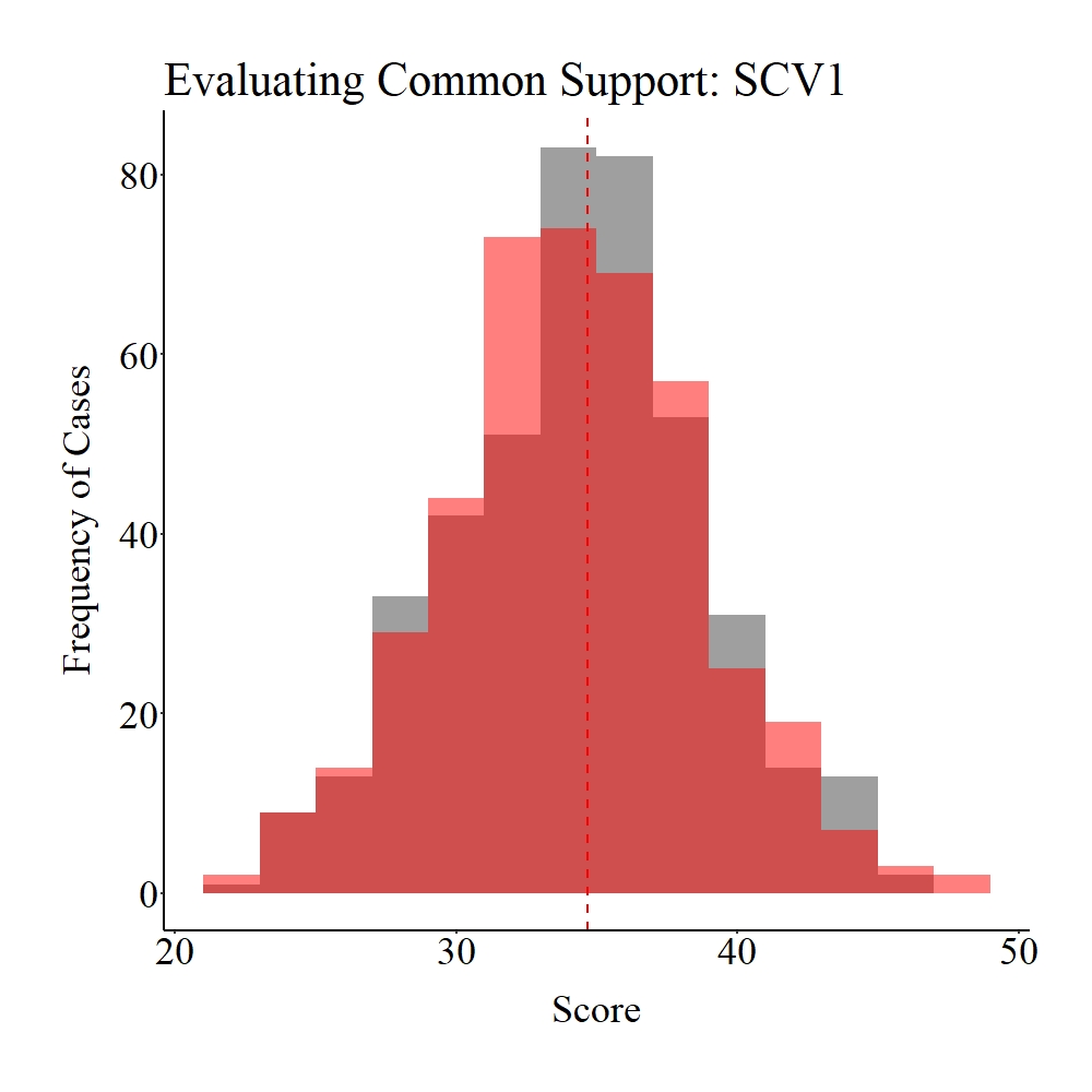
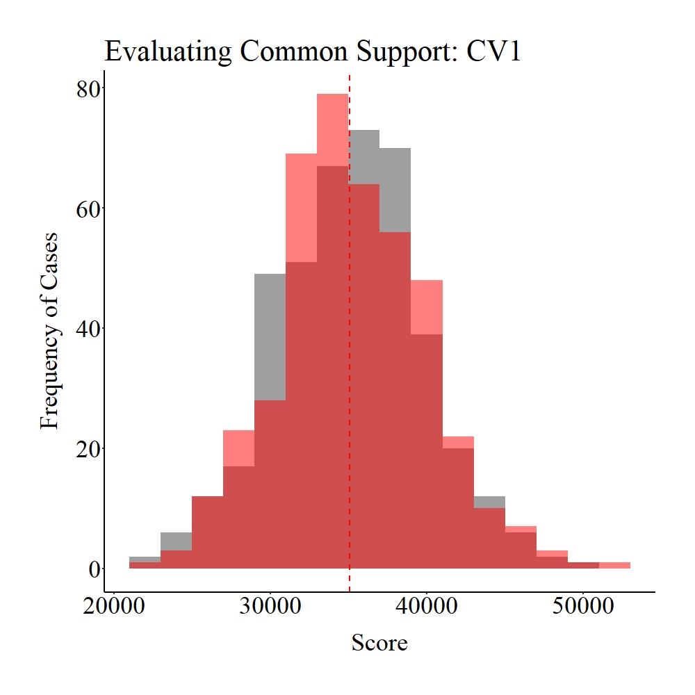
Figure Notes: The gray area represents the treatment cases only, the light red area represents the control cases only, and the dark red represents the overlap between the groups.
Additionally, the effects of Y regressed on TDI using the matched sample is closer to the true effects (-1.45) than the bivariate model estimated during our initial check (5.40). Nevertheless, -1.45 is the opposite direction and pretty far from the true estimate .50. This is because it is highly inefficient to match using variables with large distributional spans like CV1. If you were conducting this matching procedure for an evaluation, you would have to transform SCV1 and CV1 to restrict the distribution and increase the efficacy of the matching procedure.[ii]
> ### Post matching Analysis ####
>
> PMRM<-lm(Y~TDI, data = M1DF)
> summary(PMRM)

Call:
lm(formula = Y ~ TDI, data = M1DF)

Residuals:
    Min      1Q  Median      3Q     Max
-127.26  -31.74   -1.27   29.85  158.81

Coefficients:
            Estimate Std. Error t value            Pr(>|t|)
(Intercept)   353.32       2.27  155.43 <0.0000000000000002 ***
TDI            -1.45       3.21   -0.45                0.65
---
Signif. codes:  0 ‘***’ 0.001 ‘**’ 0.01 ‘*’ 0.05 ‘.’ 0.1 ‘ ’ 1

Residual standard error: 47 on 852 degrees of freedom
Multiple R-squared:  0.000237,	Adjusted R-squared:  -0.000936
F-statistic: 0.202 on 1 and 852 DF,  p-value: 0.653

>
No Support
To simulate data without any support between the treatment and control groups, we will have to alter our simulation process slightly. The easiest way to proceed is by simulating the treatment cases and the control cases separately, merging the datasets, and then generating the outcome of interest (Y). For the 500 treatment cases, SCV1 was specified to be a normally distributed variable with a mean of 0 and standard deviation of 5, while CV1 was specified to be a normally distribution variable with a mean of 80000 and a standard deviation of 5000. Given that this dataframe represented the treatment cases, all of the cases were exposed to the treatment (i.e., received a value of “1” on TDI).
> ### Treatment Cases ####
> N<-500
> set.seed(23733)
> SCV1<-trunc(rnorm(N,0,5)) # Semi-continuous Variable
> set.seed(29204)
> CV1<-trunc(rnorm(N,80000,5000)) # Continuous Variable
> TDI<-rep(1,N)
>
> TData<-data.frame(TDI,SCV1,CV1)
We replicated the process of the control cases, except SCV1 was specified to be a normally distributed variable with a mean of 70 and standard deviation of 5, while CV1 was specified to be a normally distribution variable with a mean of 20000 and a standard deviation of 5000. Moreover, none of the control cases were exposed to the treatment (i.e., received a value of “0” on TDI).
### Control Cases ####
N<-500
set.seed(23733)
SCV1<-trunc(rnorm(N,70,5)) # Semi-continuous Variable
set.seed(29204)
CV1<-trunc(rnorm(N,20000,5000)) # Continuous Variable
TDI<-rep(0,N)

CData<-data.frame(TDI,SCV1,CV1)
Given that we used the same variable names in the same order for the dataframes, we can easily merge the dataframes using the rbind command (row combined). The rbind command simply stacks one dataframe on top of the other dataframe. After creating the merged dataframe, we can generate the dependent variable (Y), which was specified to equal .50 * TDI, .01 * SCV1, and .01 * CV1. Our checks for the data simulations, similar to the previous simulation, illustrate that the bivariate association between Y and TDI is heavily biased, while the specification including the confounding variables SCV1 and CV1 produces the true slope coefficient.[iii]
> ### Combined data frames ####
>
> Data<-rbind(TData,CData)
>
> ### Creating Dependent Variable ####
>
>
> Data$Y<-.50*Data$TDI+.01*Data$SCV1+.01*Data$CV1
> ### Checking Simulations ####
>
> lm(Y~TDI, data = Data)

Call:
lm(formula = Y ~ TDI, data = Data)

Coefficients:
(Intercept)          TDI
        203          600

> lm(Y~TDI+SCV1+CV1, data = Data)

Call:
lm(formula = Y ~ TDI + SCV1 + CV1, data = Data)

Coefficients:
      (Intercept)                TDI               SCV1                CV1
0.000000000000193  0.500000000000942  0.009999999999993  0.010000000000000

>
Now let’s evaluate the common support in the population. As you probably guessed – and consistent with the data specifications –, there is no distributional overlap on SCV1 and CV1 between the treatment (gray) and control (light red) groups.
Panel A
Panel B
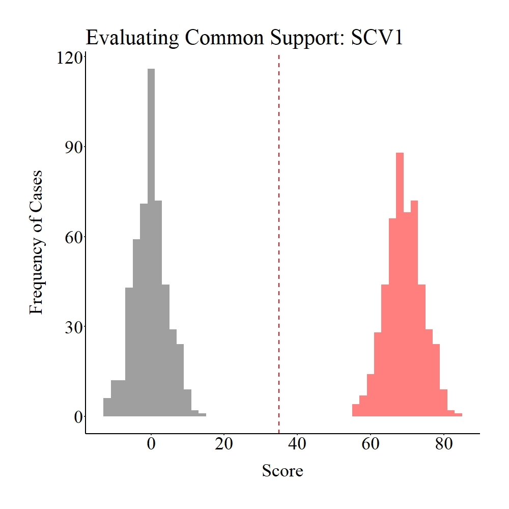
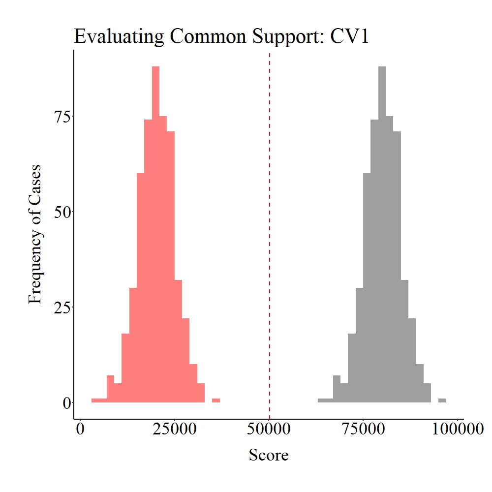
Figure Notes: The gray area represents the treatment cases only, the light red area represents the control cases only, and the dark red represents the overlap between the groups.
If we try to match treatment and control cases, we get a nice error (see the Syntax). I shouldn’t say nice error, R produces errors in red font which always brings me back to the days of being evaluated by professors. Although the error seems like gibberish, it provides us with the indication that none of our treatment cases could have been matched to our control cases using our matching requirements (i.e., nearest neighbor, random, 1 to 1, without replacement, and with a caliper of .05). We would be able to match every treatment case to a control case if we removed the caliper requirement, but that would defeat the purpose of propensity score matching. Considering that no matches were produced, we have no post-matching balance to evaluate (Yay! I guess).
> ### Matching (Nearest Neighbor, Random, 1 to 1) one time all variables ####
>
> set.seed(1992)
> M1<-matchit(TDI~SCV1+CV1, data = Data,
+             method = "nearest", m.order = "random", ratio = 1, replace = FALSE, caliper = .05)
Error in if (sum(weights) == 0) stop("No units were matched.", call. = FALSE) else if (sum(weights[treat ==  :
  missing value where TRUE/FALSE needed
In addition: Warning message:
glm.fit: algorithm did not converge
>
> summary(M1)
Error in summary(M1) : object 'M1' not found
Weak Support
No support (the example above), however, can not bias your post-matching estimates because you will not be able to match the treatment and control cases. Nevertheless, weak common support will bias post-matching estimates, as well as on occasion result in interpretations not indicative of the reality. To demonstrate this, let’s replicate the data simulation from the preceding example but specify some distributional overlap to exist between the treatment and control groups. SCV1 is specified to have a mean of 40 and standard deviation of 5 for the treatment group and a mean of 50 and a standard deviation of 5 for the control group. Similarly, CV1 is specified to have a mean of 50000 and standard deviation of 5000 for the treatment group and a mean of 40000 and a standard deviation of 5000 for the control group. The remainder of the data simulation succeeding the specifications of SCV1 and CV1 is identical to the preceding example.
> ### Treatment Cases ####
> N<-500
> set.seed(23733)
> SCV1<-trunc(rnorm(N,40,5)) # Semi-continuous Variable
> set.seed(29204)
> CV1<-trunc(rnorm(N,50000,5000)) # Continuous Variable
> TDI<-rep(1,N)
>
> TData<-data.frame(TDI,SCV1,CV1)
>
> ### Control Cases ####
> N<-500
> set.seed(23733)
> SCV1<-trunc(rnorm(N,50,5)) # Semi-continuous Variable
> set.seed(29204)
> CV1<-trunc(rnorm(N,40000,5000)) # Continuous Variable
> TDI<-rep(0,N)
>
> CData<-data.frame(TDI,SCV1,CV1)
>
> ### Combined data frames ####
>
> Data<-rbind(TData,CData)
>
> ### Creating Dependent Variable ####
>
>
> Data$Y<-.50*Data$TDI+.01*Data$SCV1+.01*Data$CV1
>
>
>
> ### Checking Simulations ####
>
> lm(Y~TDI, data = Data)

Call:
lm(formula = Y ~ TDI, data = Data)

Coefficients:
(Intercept)          TDI
        403          100

> lm(Y~TDI+SCV1+CV1, data = Data)

Call:
lm(formula = Y ~ TDI + SCV1 + CV1, data = Data)

Coefficients:
      (Intercept)                TDI               SCV1                CV1
-0.00000000000016   0.49999999999979   0.01000000000000   0.01000000000000

>
As it can be observed below, while common support (dark red) does exist between the treatment (gray) and control (light red) groups, the number of cases that fall into the region of common support is quite limited compared to the overall sample size (N = 1,000). I define this condition – some might disagree – as weak common support between the treatment and control groups.
Panel A
Panel B
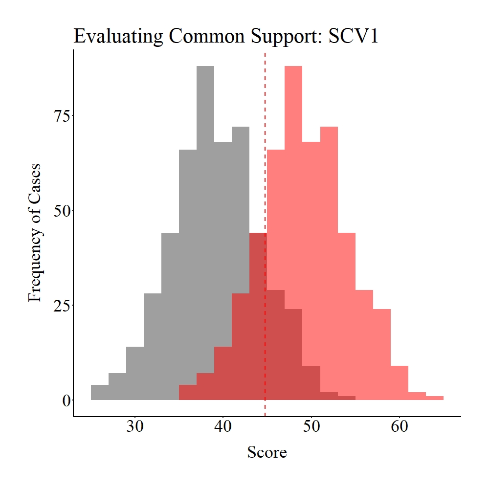
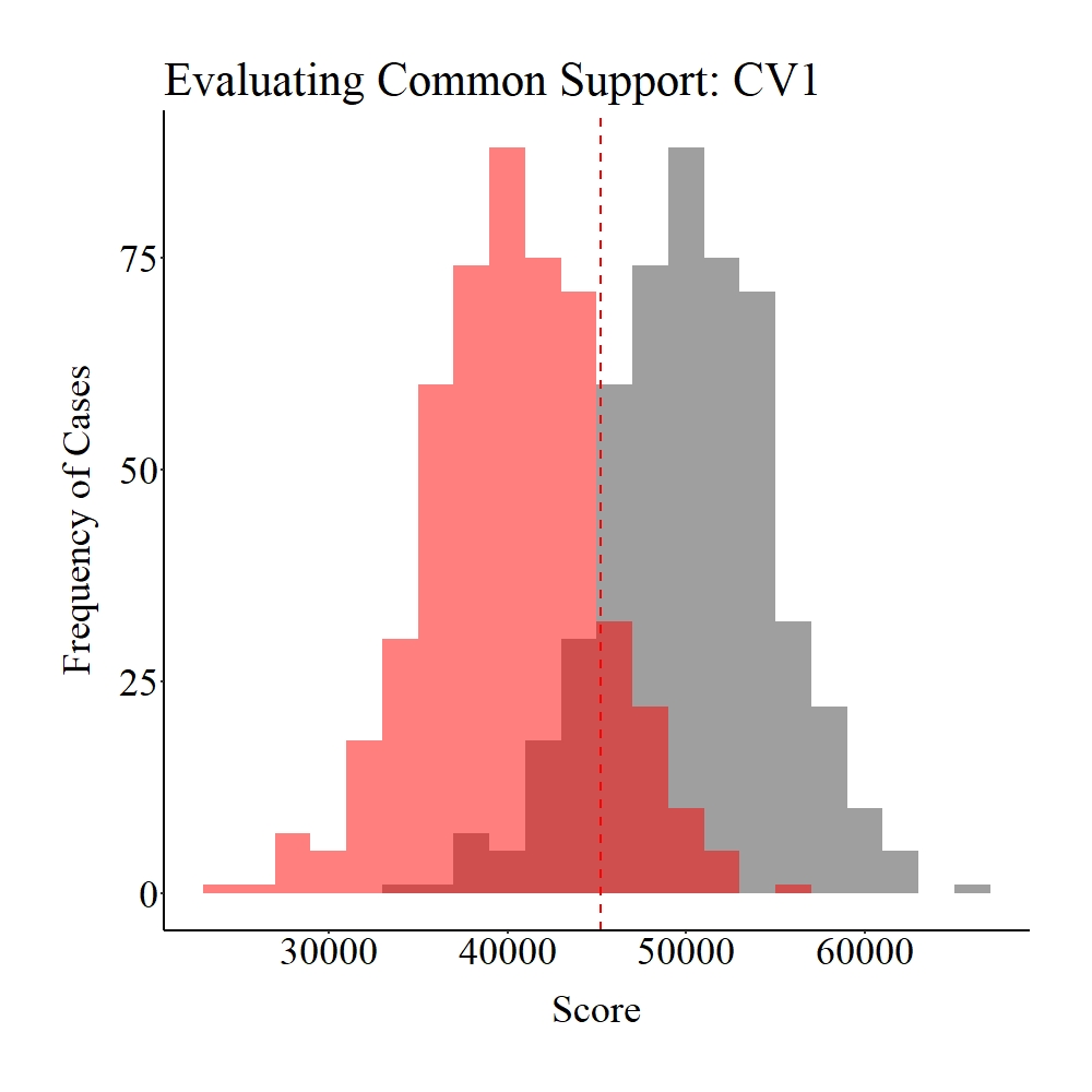
Figure Notes: The gray area represents the treatment cases only, the light red area represents the control cases only, and the dark red represents the overlap between the groups.
Unsurprisingly, the weak common support between the treatment and control group influences the efficacy of the matching procedure. Explicitly, our matching procedure below only matched 70 treatment cases to 70 control cases.
> ### Matching (Nearest Neighbor, Random, 1 to 1) one time all variables ####
>
> set.seed(1992)
> M1<-matchit(TDI~SCV1+CV1, data = Data,
+             method = "nearest", m.order = "random", ratio = 1, replace = FALSE, caliper = .05)
>
> summary(M1)

Call:
matchit(formula = TDI ~ SCV1 + CV1, data = Data, method = "nearest",
    replace = FALSE, m.order = "random", caliper = 0.05, ratio = 1)

Summary of Balance for All Data:
         Means Treated Means Control Std. Mean Diff. Var. Ratio eCDF Mean eCDF Max
distance         0.896         0.104           3.882      1.007     0.481     0.86
SCV1            39.734        49.734          -1.993      1.000     0.256     0.69
CV1          50238.066     40238.066           2.097      1.000     0.430     0.74


Summary of Balance for Matched Data:
         Means Treated Means Control Std. Mean Diff. Var. Ratio eCDF Mean eCDF Max
distance         0.506         0.503           0.013      1.018     0.002    0.029
SCV1            44.657        45.200          -0.108      1.188     0.018    0.114
CV1          45093.129     45541.800          -0.094      1.248     0.029    0.100
         Std. Pair Dist.
distance           0.029
SCV1               0.740
CV1                0.714

Percent Balance Improvement:
         Std. Mean Diff. Var. Ratio eCDF Mean eCDF Max
distance            99.7     -144.5      99.5     96.7
SCV1                94.6        N/A      93.1     83.4
CV1                 95.5        N/A      93.2     86.5

Sample Sizes:
          Control Treated
All           500     500
Matched        70      70
Unmatched     430     430
Discarded       0       0

>
> M1DF<-match.data(M1)
>
Taking a moment to explore the balance in the matched sample, it appears that only treatment and control participants within the common support region were matched to each other (see pre-matching figures). Given that the region of common support represents unique cases in each distribution (> 1 standard deviation from the mean), it is likely that our post-matching estimates will be biased.
Panel A
Panel B
Panel C
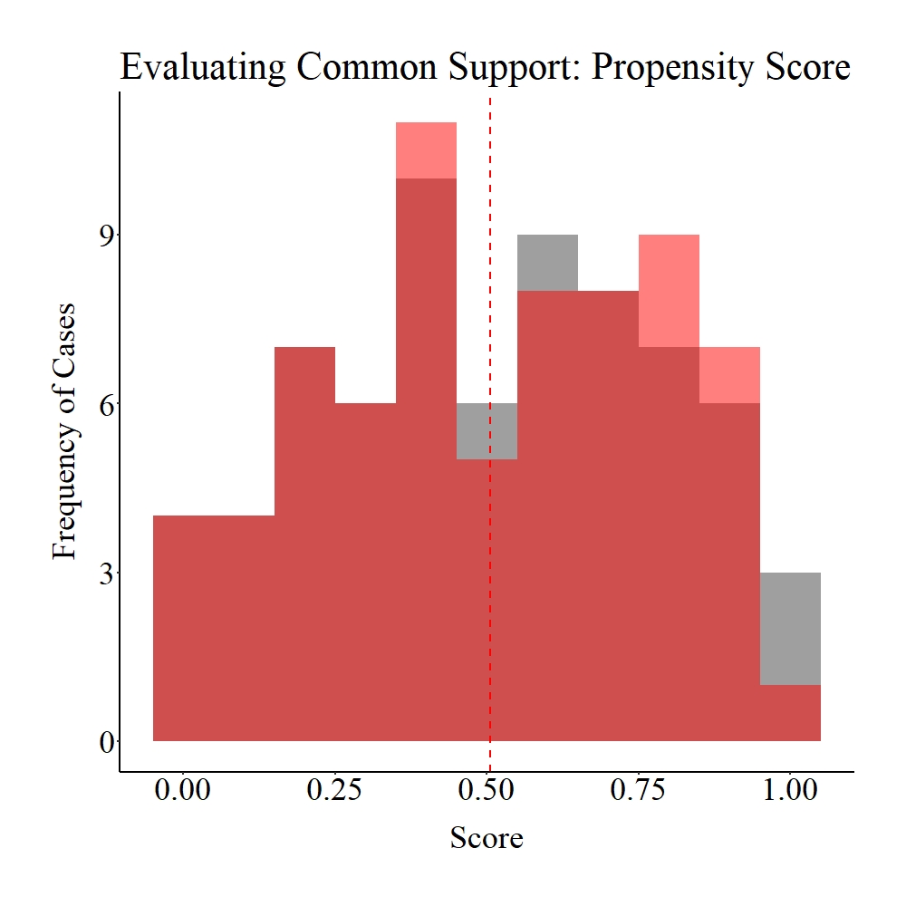
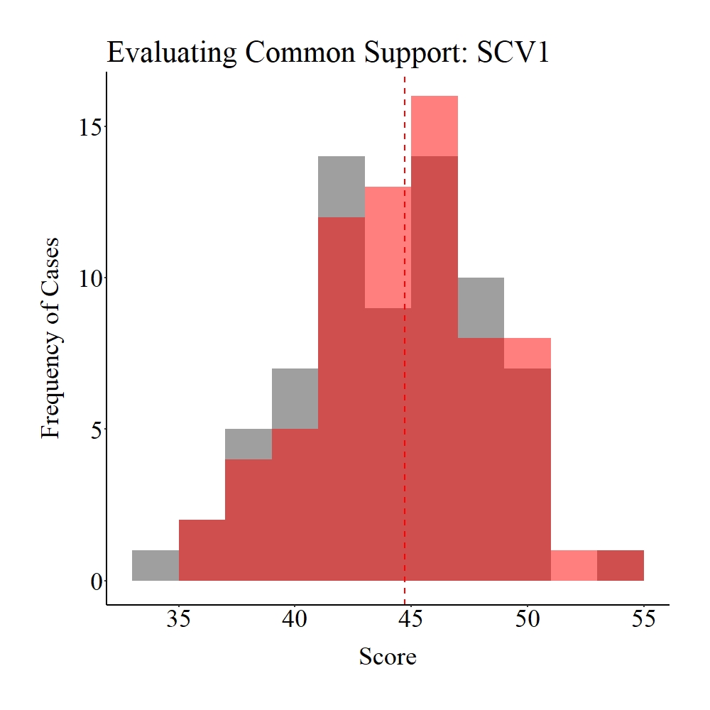
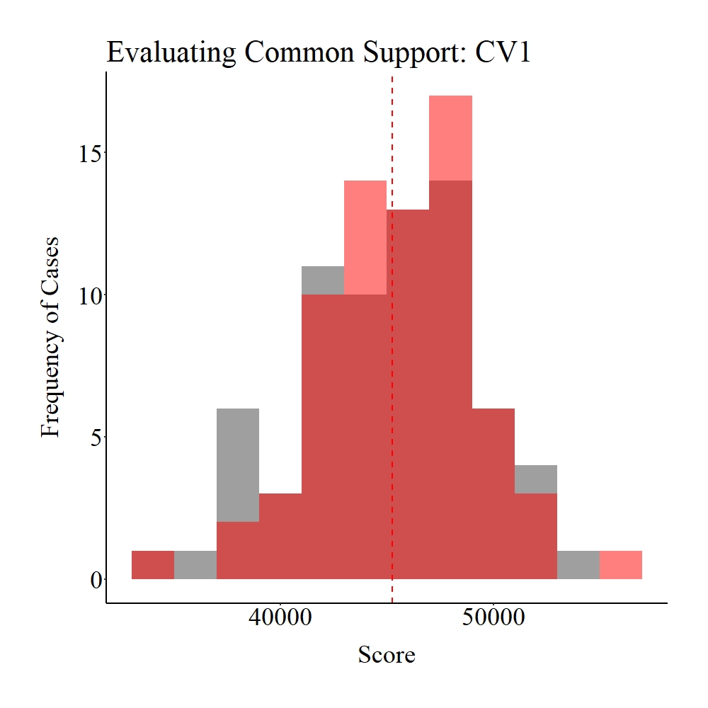
Figure Notes: The gray area represents the treatment cases only, the light red area represents the control cases only, and the dark red represents the overlap between the groups.
As suspected our post-matching evaluation yielded results suggesting a bivariate association between Y and TDI of -3.99 and the results are not statistically significant. These estimates suggest that the matching procedure was inefficient, as well as resulted in findings that are a meaningful departure from the true association.
> ### Post matching Analysis ####
>
> PMRM<-lm(Y~TDI, data = M1DF)
> summary(PMRM)

Call:
lm(formula = Y ~ TDI, data = M1DF)

Residuals:
    Min      1Q  Median      3Q     Max
-123.78  -25.01    1.06   25.25  106.41

Coefficients:
            Estimate Std. Error t value            Pr(>|t|)
(Intercept)   455.87       4.73    96.4 <0.0000000000000002 ***
TDI            -3.99       6.69    -0.6                0.55
---
Signif. codes:  0 ‘***’ 0.001 ‘**’ 0.01 ‘*’ 0.05 ‘.’ 0.1 ‘ ’ 1

Residual standard error: 39.5 on 138 degrees of freedom
Multiple R-squared:  0.00258,	Adjusted R-squared:  -0.00465
F-statistic: 0.357 on 1 and 138 DF,  p-value: 0.551

>
Conclusions
The assumption of common support is imperative to the efficacy of propensity score matching. Explicitly, you can not match cases on key covariates if distributional overlap does not exist between the treatment and control groups. Nevertheless, the biggest concern should exist when weak common support is observed between the treatment and control groups on the matching covariates. When weak common support is observed, the post-matching estimates can become biased and result in interpretations not representative of reality. As such, it is important to visually explore the distributional overlap between the treatment and control groups before conducting any matching procedures. If there is weak – or even moderate – common support, transforming the matching variables of interest could increase the common support between the treatment and control groups. Next entry will review the post-matching bias created when we exclude treatment cases during the matching procedure.
[i] To truly evaluate balance, it is best to generate and interpret the key statistics, as well as create the visual plots.
[ii] The efficacy of each matching procedure will be discussed in detail in a future entry of the Violating Assumption Series.
[iii] The relationship between Y and TDI in the no support and weak support examples is confounded by SCV1 and CV1 because of the way we generated the data. Instead of the traditional confounding specification where TDI is specified to equal SCV1 and CV1, confounding effects can be created when the distributional specifications for SCV1 and CV1 differ between the separately simulated treatment and control groups.
License: Creative Commons Attribution 4.0 International (CC By 4.0)
