1. Introduction (PDF & R-Script)
Across the social sciences (besides psychology), the development of valid measures is often sacrificed in an effort to implement a randomized controlled trial or produce results generalizable to a population of interest. Sacrificing measurement, however, creates problems not only by reducing our ability to accurately capture the variation in a concept, but also limits our ability to observe the true statistical association between concepts. If one or more of our concepts are not properly operationalized – i.e., the variation in the measure does not capture the variation in the population – the estimates derived from any general linear model will become biased.[i] The preceding entries directly demonstrated this source of statistical bias by altering the level of measurement of an observed construct. Nonetheless, many constructs in the social sciences cannot be directly observed. For example, we cannot directly observe an individual’s risk of recidivism, psychological status, or desire to spend money. Considering how many unobserved constructs permeate the social science literature, it is important to expand our preceding discussions to include conversations about the creation of measures that capture variation associated with observed and unobserved concepts.
Briefly, by my own definition, measurement creation is the process of combining observed items to capture the variation associated with a well-defined observed or unobserved – latent – construct. For example, one method of measuring involvement in criminal behavior is the aggregate number of offenses an individual has committed. Although we can directly request respondents to report the number of crimes they have previously committed, oftentimes we request respondents to report the number of times they committed crime X, crime Y, and crime z. Or, better yet, we only have access to official data that records the number of times an individual has been arrested for violent offenses, drug offenses, other offenses, etc. In these situations, we are required to create a measure capturing the variation in the aggregate number of offenses an individual has committed using the available items. Although for this example we would simply add up each of the existing measures to capture the aggregate number of offenses an individual has committed, a variety of techniques can be implemented to create measures. This entry will review how existing items can be integrated into the development of a dichotomous indicator (e.g., diagnosis), 2) ordered indicator (e.g., scaled diagnosis), 3) aggregate scale (e.g., number of events), and 4) variety score when capturing the variation in an unobserved concept. Throughout these examples, we will review the conceptualization and operationalization when creating each of these measures, as well as how each technique influences the statistical associations within a three-variable system.
2. My Background
It is important to start off by stating I am not an expert on theoretical frameworks for measurement creation. While I possess a comprehensive understanding of how to conduct a psychometric evaluation and the analytical techniques used to conduct these evaluations, I have limited working knowledge of the theoretical process used to create items/questions that tap observed or unobserved constructs. This is because I was trained as a quantitative criminologist, where we rely on the justification of “someone has published with this measure before me” to explain how items tap variation in observed or unobserved constructs. This justification, as you might suspect, is flawed. However, it is a good thing that this entry will not focus on the theoretical process of item/question creation – or item response theory –, but rather focus on the process of recoding a series of items/questions into a single variable. Although my knowledge of theory is limited when discussing measurement, I am a major proponent of the argument that theory – and to some degree the data collection process – should always guide the development of items/questions and the creation of a single variable from a series of items/questions. You should never allow your data to guide measurement creation alone (looking at you machine learning)! Okay, I shouldn’t just blame machine learning, but you get the idea.
3. Capturing Variation Associated with Observed and Unobserved Constructs (The Basics)
A variety of techniques can be used to recode a series of items into a single variable intended to capture the variation in an observed or unobserved concept. Briefly, when I use the term item or question, I am referring to measures collected during the administration of a survey or during official data collection. Importantly, items and questions capture variation associated with concepts or sub-concepts that can be directly observed. For example, if we were interested in the concept of income,[ii] we can administer a survey requesting respondents to report their yearly earnings. While most conceptualizations of income can be directly operationalized by requesting respondents to answer a single question, we can ask a series of questions to better understand the sources of income across the population. For example, we can ask respondents to report their yearly earnings from 1) their employment, 2) stocks, 3) bonds, 4) retirement accounts, and 5) other assets. The respondents’ answers to these questions can then be used to create a measure of total income.
Another example would be the process of capturing variation associated with the variety of different criminal activities an individual committed. For instance, the variety of different criminal activities an individual committed can be captured using a single item or captured using multiple items. A single item approach would simply request respondents to report how many different types of crimes they engaged in over the past year. However, we can also capture variation associated with how many different types of crimes an individual committed by requesting them to report how many times they committed crime x, crime y, and crime z. Using these items, we could create dichotomous indicators identifying if an individual committed each of the specified criminal activities, which can then be aggregated to capture how many different types of crimes an individual committed.
An unobserved construct represents a concept that cannot be directly captured using a survey or official data source. Unobserved constructs require the combination of items to capture the variation that is expected to be associated with the construct. For instance, general intelligence cannot be directly measured. As such, to capture the variation expected to be associated with general intelligence, answers to a variety of items must be combined in a systematic manner. Tools that are designed to capture general intelligence commonly rely on a series of items tapping an individual’s verbal and math aptitude, as well as creativity, reasoning, logic, and processing abilities.
4. Bias and Measurement Creation (Considering the Variation Captured)
Measurement creation is a tedious process requiring one to clearly define and theoretically justify the concept being measured, while also developing an operationalization that accurately captures the variation associated with the concept of interest. The difference between the conceptualization and the operationalization of a concept is a major source of statistical bias. In particular, if the operationalization does not capture the variation expected to be associated with the concept defined for a population, all the statistical models included the measure will become biased. The process of aligning the conceptualization and operationalization of a construct becomes more difficult when combining multiple items to create a measure which, in turn, increases the likelihood of statistical associations becoming biased.
While a major source of bias is the disjunction between the conceptualization and operationalization of a concept, measurement error can contribute to the observation of findings not representative of reality. Briefly, measurement error can be defined as the difference between the measured score on a concept and the true score on a concept. For instance, the difference between an individual’s true height of 5’6.75” and the measured height of 5’6” is measurement error — I swear this example is unrelated to my height. Measurement error can be systematic (e.g., caused by a poorly asked question) and/or random. The existence of systematic measurement error means that the operationalization of a concept cannot accurately capture the variation associated with that concept in a non-random manner across the population. For example, rounding the weight of participants to the nearest whole number in pounds (e.g., 165 lbs.) means that there is a finite, but systematic, error in the measurement of weight. Measurement error would exist in this example because the weight of only a limited number of people would be perfectly captured by whole numbers.
The existence of random measurement error means that the operationalization of a concept does not accurately capture the variation associated with that concept in a random manner across the population. For example, if we measured everyone’s height and due to some non-systematic process, the measured height of some individuals was not equal to their true height.
Measurement error exists in every operationalization due to the inability to create a perfect measure for a concept. This is true for both the hard sciences and the social sciences, with the latter being impacted more due to a diminished ability to create tools that accurately measure human phenomena. Importantly, measurement error is exacerbated when combining items and questions. That is, the variation in items/questions associated with measurement error is combined when multiple items are used to operationalize an observed or unobserved concept. The proportion of the variation attributed to measurement error is conditional upon the measurement error in each item and the process used to combine the items/questions. This means, that in addition to the bias generated by the disjunction between the conceptualization and operationalization of a construct, additional bias can be observed in statistical estimates due to the combination of measurement error across observed items. As demonstrated in the simulations below, the conceptualization and operationalization of a construct, as well as measurement error, can directly influence the statistical associations observed between constructs and, more importantly, have important implications for the conclusions drawn from statistical evaluations.
5. The Simulated Example
A three variable system was created to evaluate the effects of distinct operationalizations for a construct on the statistical associations observed when subjecting the system to a path model. As displayed in Figure 1, the three variable system was specified where variation in A caused variation in both X and Y, and variation in X caused variation in Y. The variation in A was specified to be a gamma distribution with a shape of 2 and rate of .1, while the residual variation in X and Y was specified to be normally distributed with a mean of 0 and standard deviation of 20 and 30 (respectively). The linear slope of the association between A and X was specified to be .2, the linear slope of the association between A and Y was specified to be 4, and the linear slope of the association between X and Y was specified to be 1 (as indicated in the R-code below).
[Figure 1]

> n<-10000
>
> set.seed(1992)
> A<-rgamma(n, shape = 2, rate = .1) # A Represents a Latent Construct (Unobservable)
> summary(A)
         Min.       1st Qu.        Median          Mean       3rd Qu.          Max.
  0.151734682   9.609991566  16.682445020  20.063699482  27.052281510 132.738427433
> X<-.2*A+rnorm(n,0,20)
> cor(A,X)
[1] 0.138787713631
> Y<-X+.4*A+rnorm(n,0,30)
> cor(A,Y)
[1] 0.237466159495
> cor(X,Y)
[1] 0.571791664967
>
Let’s add some labels to the three variable system to help us understand how the operationalization of a construct influences the interpretations derived from a model. First, and foremost, let’s imagine that X is the number of days using substances and Y is weeks unemployed. Now, let’s imagine A represents the number of days an individual experienced severe depression during the year. In this context, severe depression is a latent construct conceptualized as a serious mood disorder corresponding with the persistent expression of symptoms associated with depression. As an unobserved latent construct, we cannot directly measure the number of days an individual experienced severe depression, but we can measure the number of days an individual experienced symptoms associated with severe depression. Given this, we developed an assessment capturing variation in the number of days individuals felt: 1) sad and lonely, 2) unable to get out of bed, 3) like nothing could cheer them up, 4) unmotivated to do anything, 5) unhappy with their current situation, 6) a loss of appetite, 7) no pleasure in hobbies and activities they previously enjoyed, 8) the world would be better off without them, 9) their life was spiraling out of control, and 10) that all they could do was sleep. The measurement model for the number of days experiencing severe depression is illustrated in Figure 2.
[Figure 2]
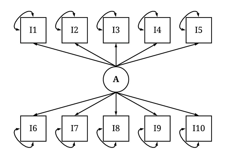
The process of simulating a latent construct requires us to simulate a variable representative of the unobserved construct and then use that variable to cause variation in a series of variables representative of the observed items. Following this process, A was specified to predict variation in Items 1-10, where the items were initially coded as continuous constructs. The causal influence of A on Items 1-10 was specified to be linear, where the slope of the association would be 10 (not really important information when discussing the process of simulating latent constructs). The residual variation in each construct was then specified to be normally distributed with a mean of 0 and a standard deviation of 50 (5* rnorm(n,0,10)). After creating the continuous measures of Items 1-10, the scores on the items were normalized – to emulate a probability. After normalizing the measures, values were drawn from a gamma distribution using the inverse of the probability (1-I#_P) to ensure that the values on Items 1-10 would emulate real data measures of the number of days an individual experienced depressive symptoms over a year. Given our constraint to 1-year, the scores on Items 1-10 were top coded at 365.
> I1_C<-10*A+5*rnorm(n,0,10)
> I1_P<-((I1_C)-min(I1_C-1))/((max(I1_C+1))-min(I1_C-1))
> I2_C<-10*A+5*rnorm(n,0,10)
> I2_P<-((I2_C)-min(I2_C-1))/((max(I2_C+1))-min(I2_C-1))
> I3_C<-10*A+5*rnorm(n,0,10)
> I3_P<-((I3_C)-min(I3_C-1))/((max(I3_C+1))-min(I3_C-1))
> I4_C<-10*A+5*rnorm(n,0,10)
> I4_P<-((I4_C)-min(I4_C-1))/((max(I4_C+1))-min(I4_C-1))
> I5_C<-10*A+5*rnorm(n,0,10)
> I5_P<-((I5_C)-min(I5_C-1))/((max(I5_C+1))-min(I5_C-1))
> I6_C<-10*A+5*rnorm(n,0,10)
> I6_P<-((I6_C)-min(I6_C-1))/((max(I6_C+1))-min(I6_C-1))
> I7_C<-10*A+5*rnorm(n,0,10)
> I7_P<-((I7_C)-min(I7_C-1))/((max(I7_C+1))-min(I7_C-1))
> I8_C<-10*A+5*rnorm(n,0,10)
> I8_P<-((I8_C)-min(I8_C-1))/((max(I8_C+1))-min(I8_C-1))
> I9_C<-10*A+5*rnorm(n,0,10)
> I9_P<-((I9_C)-min(I9_C-1))/((max(I9_C+1))-min(I9_C-1))
> I10_C<-10*A+5*rnorm(n,0,10)
> I10_P<-((I10_C)-min(I10_C-1))/((max(I10_C+1))-min(I10_C-1))
> # Items ####
>
>
> Item1<-rgamma(n, shape = 2, rate = 1-I1_P)
> summary(Item1)
         Min.       1st Qu.        Median          Mean       3rd Qu.          Max.
   0.02396641    1.24012426    2.17062739    2.93697532    3.52659164 2866.49780753
> Item2<-rgamma(n, shape = 2, rate = 1-I2_P)
> summary(Item2)
         Min.       1st Qu.        Median          Mean       3rd Qu.          Max.
   0.02072410    1.27547404    2.22108368    2.95334682    3.61590732 2479.22231827
> Item3<-rgamma(n, shape = 2, rate = 1-I3_P)
> summary(Item3)
          Min.        1st Qu.         Median           Mean        3rd Qu.           Max.
   0.012895928    1.252431063    2.212495380    2.829538858    3.595902395 1195.500537402
> Item4<-rgamma(n, shape = 2, rate = 1-I4_P)
> summary(Item4)
         Min.       1st Qu.        Median          Mean       3rd Qu.          Max.
  0.026426924   1.234009573   2.163373560   2.697607687   3.491203343 528.670558826
> Item5<-rgamma(n, shape = 2, rate = 1-I5_P)
> summary(Item5)
          Min.        1st Qu.         Median           Mean        3rd Qu.           Max.
   0.017237008    1.255052086    2.180020785    2.847608448    3.531661541 1879.047304852
> Item6<-rgamma(n, shape = 2, rate = 1-I6_P)
> summary(Item6)
         Min.       1st Qu.        Median          Mean       3rd Qu.          Max.
   0.02696725    1.27441900    2.24981169    3.04359311    3.63680078 3265.28725631
> Item7<-rgamma(n, shape = 2, rate = 1-I7_P)
> summary(Item7)
         Min.       1st Qu.        Median          Mean       3rd Qu.          Max.
   0.00959981    1.23096154    2.16203758    3.06245403    3.52588171 4229.03223338
> Item8<-rgamma(n, shape = 2, rate = 1-I8_P)
> summary(Item8)
         Min.       1st Qu.        Median          Mean       3rd Qu.          Max.
   0.01762628    1.25947747    2.25155304    3.15378716    3.64752224 4269.78767835
> Item9<-rgamma(n, shape = 2, rate = 1-I9_P)
> summary(Item9)
         Min.       1st Qu.        Median          Mean       3rd Qu.          Max.
  0.013728806   1.230842773   2.172124944   2.740608844   3.553298981 903.406985272
> Item10<-rgamma(n, shape = 2, rate = 1-I10_P)
> summary(Item10)
         Min.       1st Qu.        Median          Mean       3rd Qu.          Max.
  0.020194961   1.235167831   2.172981364   2.694630420   3.523753471 550.215582977
>
> Item1[Item1>365]<-365
> Item2[Item2>365]<-365
> Item3[Item3>365]<-365
> Item4[Item4>365]<-365
> Item5[Item5>365]<-365
> Item6[Item6>365]<-365
> Item7[Item7>365]<-365
> Item8[Item8>365]<-365
> Item9[Item9>365]<-365
> Item10[Item10>365]<-365
Okay, so that block of R-code is really long. So, let’s focus on how the variation in Items 1-10 are associated with the variation in the latent construct A – severe depression. Below is the correlation matrix of the 10 items plus X, Y, and A. Focusing on the bivariate association between A and Items 1-10, it can be observed that A is correlated with each of the items. Those correlations, however, are nominal due to the influence of A on the items and the measurement error that exists in the items. Overall, however, the bivariate correlations between Items 1-10 suggests that the items are capturing variation in a similar construct.
> corr.test(DF)
Call:corr.test(x = DF)
Correlation matrix
          X    Y    A Item1 Item2 Item3 Item4 Item5 Item6 Item7 Item8 Item9 Item10
X      1.00 0.57 0.14  0.03  0.02  0.02  0.02  0.02  0.01  0.01  0.02  0.02   0.01
Y      0.57 1.00 0.24  0.04  0.04  0.05  0.04  0.05  0.04  0.04  0.04  0.04   0.03
A      0.14 0.24 1.00  0.18  0.19  0.20  0.18  0.19  0.19  0.18  0.20  0.18   0.17
Item1  0.03 0.04 0.18  1.00  0.78  0.78  0.79  0.78  0.78  0.79  0.78  0.79   0.78
Item2  0.02 0.04 0.19  0.78  1.00  0.77  0.78  0.78  0.78  0.79  0.77  0.78   0.78
Item3  0.02 0.05 0.20  0.78  0.77  1.00  0.78  0.78  0.78  0.78  0.78  0.78   0.78
Item4  0.02 0.04 0.18  0.79  0.78  0.78  1.00  0.78  0.78  0.78  0.78  0.78   0.78
Item5  0.02 0.05 0.19  0.78  0.78  0.78  0.78  1.00  0.78  0.79  0.78  0.78   0.79
Item6  0.01 0.04 0.19  0.78  0.78  0.78  0.78  0.78  1.00  0.78  0.77  0.78   0.78
Item7  0.01 0.04 0.18  0.79  0.79  0.78  0.78  0.79  0.78  1.00  0.78  0.78   0.79
Item8  0.02 0.04 0.20  0.78  0.77  0.78  0.78  0.78  0.77  0.78  1.00  0.77   0.78
Item9  0.02 0.04 0.18  0.79  0.78  0.78  0.78  0.78  0.78  0.78  0.77  1.00   0.79
Item10 0.01 0.03 0.17  0.78  0.78  0.78  0.78  0.79  0.78  0.79  0.78  0.79   1.00
5.1 True Model (Treating Severe Depression as Observed)
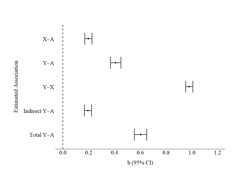
Now that we have coded our measures, let’s estimate the baseline effects of A on X and Y. For this model, we will treat A (number of days with severe depression) as an observed construct and use it to predict the variation in X (number of days using substances) and Y (weeks unemployed). This model will provide us with an understanding of the magnitude and direction of the statistical associations between A, X, and Y when we capture all the variation in A and A is conceptualized as a continuous construct. In the model specified below (F1), the direct effects of A on X and A and X on Y were estimated, as well as the indirect effects of A on Y and the total effects of A on Y. The unstandardized slope coefficients produced by the model specified below are provided in Figure 3.
F1<-'
X~a*A
Y~b*A+c*X

# Indirect Effects
ac:=(a*c)
# Total Effects
abc:=b+(a*c)

'

M1<-sem(F1,data=DF, estimator = "ML")
SM1<-summary(M1, fit.measures= TRUE, standardized = TRUE, ci = TRUE, rsquare = T)
Evident by the estimated slope coefficients, all the associations appeared to be statistically significant in the positive direction. Of importance, a 1-point increase in A was directly associated with a .197 increase in X and a .409 increase in Y. Moreover, A had an indirect effect of .193 on Y through X. In total, a 1-point change in A was associated with a .602 change in Y.
To interpret these estimates using the substantive labels, increases in the number of days with severe depression (A) was associated with increases in the number of days using substances (X) and increases in weeks unemployed (Y). Severe depression directly influenced weeks unemployed and indirectly effected weeks unemployed by number of days an individual used substances. The magnitude of the total effects suggest that a 1-day increase in severe depression per year was associated with a .6 increase in weeks unemployed (~ 4 days) and a .2 increase in the number of days using substances. These findings, substantively, suggest that policy implications should only be developed for individuals that experience severe depression for an elongated period of time during a year.
[Figure 3]
5.2. Dichotomous Indicator
Now let’s operationalize the variation in A using Items 1-10 using distinct conceptualizations. First up, and the most commonly used technique in the social sciences, is the development of a dichotomous indicator. To briefly describe, a dichotomous indicator recodes the information from one or more observed items into a 0 or 1 scale. Dichotomous indicators are commonly used to represent diagnosis status, treatment status, the occurrence of an event, or exposure to some characteristics/event. In psychology, it is common practice to request participants to report their symptoms using a Likert scale, and then transform those items into a dichotomous indicator identifying diagnosis status. Similarly, in criminology it is commonplace to create a dichotomous indicator identifying if an individual engaged in criminal behavior (“0” = No; “1” = Yes) using a series of continuous items capturing the number of times an individual has engaged in various criminal behaviors.
For our current example, our dichotomous indicator for A will be conceptualized as “did the individual experience all of the symptoms of severe depression at some point during the past year?” Inevitably, the leniency of our conceptualization will have an impact on the operationalization of our measure. In this case, our dichotomous indicator should be operationalized where a value of “0” indicated that they did not experience all of the symptoms of severe depression at some point during the past year and a value of “1” would indicate that they did experience all the symptoms of severe depression at some point during the past year.
Given this conceptualization and operationalization, a methodological process was developed to recode the information captured by Items 1-10 into a dichotomous indicator. For this measure, we decided to provide individuals with a value of “1” on DI_A – the dichotomous indicator of A – if they experienced each of the symptoms for at least one and a half days during the year. This was coded into the computer as >= 1.5 using the & sign, meaning that an individual had to score >= 1.5 on each of the items to score a “1” on DI_A (expressed in the code below). If they did not score >= 1.5 on each of the items, the case would be assigned a value of “0” on DI_A. The coding scheme below resulted in 9,685 cases receiving a “0” and 315 cases receiving a “1.” Please note that our coding scheme does not require the participants to experience each of the symptoms during a single day but had to report that they experienced each of the symptoms for at least one day during the year.
Reminder: A variety of conceptualizations and operationalizations can be implemented to create a dichotomous indicator for A from Items 1-10, all of which will produce distinct estimates of the effects.
> ## Dichotomy Creation ####
>
> summary(DF$Item1)
        Min.      1st Qu.       Median         Mean      3rd Qu.         Max.
  0.02396641   1.24012426   2.17062739   2.68682554   3.52659164 365.00000000
>
> DF$DI_A<-0
> DF$DI_A[DF$Item1>=1.5 &
+         DF$Item2>=1.5 &
+         DF$Item3>=1.5 &
+         DF$Item4>=1.5 &
+         DF$Item5>=1.5 &
+         DF$Item6>=1.5 &
+         DF$Item7>=1.5 &
+         DF$Item8>=1.5 &
+         DF$Item9>=1.5 &
+         DF$Item10>=1.5]<-1
> table(DF$DI_A)

   0    1
9685  315
>
>
> ## Dichotomy Model ####
>
> F1<-'
+ X~a*DI_A
+ Y~b*DI_A+c*X
+
+ # Indirect Effects
+ ac:=(a*c)
+ # Total Effects
+ abc:=b+(a*c)
+
+ '
>
> M1<-sem(F1,data=DF, estimator = "ML")
> SM1<-summary(M1, fit.measures= TRUE, standardized = TRUE, ci = TRUE, rsquare = T)
>
DI_A was then subjected to a model identical to the true model. That is, DI_A was used to predict variation in X and Y, while X was also used to predict variation in Y. This model permits the estimation of the direct effects of DI_A on X and Y and the indirect effects of DI_A on Y through X. The unstandardized slope coefficients are presented in Figure 4.
As demonstrated below, the slope coefficients observed when estimating the direct effects of DI_A on X and Y were substantively different than the slope coefficients observed when estimating the direct effects of A (observed) on X and Y. The results suggest that moving from a 0 to a 1 on DI_A results in a 3.510 increase in X and an 8.482 increase in Y. The magnitude of the total effects of DI_A on Y through X was 12.054.
If we were to interpret these estimates using the substantive labels we developed, the results suggest that experiencing all the symptoms of severe depression at some point during the past year is associated with approximately 3 more days using substances and 8 to 12 more weeks unemployed. This interpretation is functionally different from the interpretation of the true model, providing a high degree of support for the development of an intervention to reduce the likelihood of individuals experiencing one and a half days of every symptomology over the course of a year.
[Figure 4]

5.3. Ordered Indicator
Now let’s replicate the previous process but conceptualize A as an ordered construct. In particular, we are going to conceptualize A as an ordered indicator of the frequency of experiencing severe depressive symptoms over the course of the year. Again, this conceptualization provides the ability to operationalize a measure of A using various coding schemes. Our ordered indicator is going to range from 1 to 4 (4-point scale), with higher values indicating that a case experienced severe depressive symptoms worse over the course of the year. Similar to dichotomous indicators, ordered indicators are frequently used in the social sciences to 1) measure constructs difficult to operationalize on continuous scales (e.g., Likert scale), 2) simplify the distribution of a construct or, 3) capture variation on multiple items within an ordered indicator.
A common example of the combination of continuous items into an ordered indicator is the creation of a BMI indicator. A BMI indicator is the combination of height and weight – often measured continuously – into a score which is then used to categorize individuals into five different body types: underweight, normal, overweight, obese, extremely obese. Scholars conducting research on BMI or using BMI as a control variable often introduce an ordered indicator into the model where “1” = underweight; “2” = normal; “3” = overweight, “4” = obese; and “5” = extremely obsess.
It was decided that cases that did not experience severe symptoms of depression would receive a “0”, if a case experienced 5 or more days of at least one symptom they would receive a “1”, if a case experienced 1 or more days of every symptom they would receive a “2”, if case experienced 10 or more days of at least one symptom they would receive a “3”, and if a case experienced 2 or more days of every symptom they would receive a “4” on the ordered indicator for A. While this coding scheme is not intuitively indicative of worse symptomology, it definitely creates a nice distribution of scores (not saying this is why I chose this coding scheme). Using the R-script below, ORD_A was created, where 3,152 cases received a “0”, 4,914 cases received a “1”, 1,247 cases received a “2”, 627 cases received a “3”, and 60 cases received a “4”
> ## Ordered Measure Creation ####
>
>
> DF$ORD_A<-0
> DF$ORD_A[DF$Item1>=5 |
+            DF$Item2>=5 |
+            DF$Item3>=5 |
+            DF$Item4>=5 |
+            DF$Item5>=5 |
+            DF$Item6>=5 |
+            DF$Item7>=5 |
+            DF$Item8>=5 |
+            DF$Item9>=5 |
+            DF$Item10>=5]<-1
> DF$ORD_A[DF$Item1>=1 &
+            DF$Item2>=1 &
+            DF$Item3>=1 &
+            DF$Item4>=1 &
+            DF$Item5>=1 &
+            DF$Item6>=1 &
+            DF$Item7>=1 &
+            DF$Item8>=1 &
+            DF$Item9>=1 &
+            DF$Item10>=1]<-2
> DF$ORD_A[DF$Item1>=10 |
+            DF$Item2>=10 |
+            DF$Item3>=10 |
+            DF$Item4>=10 |
+            DF$Item5>=10 |
+            DF$Item6>=10 |
+            DF$Item7>=10 |
+            DF$Item8>=10 |
+            DF$Item9>=10 |
+            DF$Item10>=10]<-3
> DF$ORD_A[DF$Item1>=2 &
+            DF$Item2>=2 &
+            DF$Item3>=2 &
+            DF$Item4>=2 &
+            DF$Item5>=2 &
+            DF$Item6>=2 &
+            DF$Item7>=2 &
+            DF$Item8>=2 &
+            DF$Item9>=2 &
+            DF$Item10>=2]<-4
> table(DF$ORD_A)

   0    1    2    3    4
3152 4914 1247  627   60
>
>
> ## Ordered Model ####
>
> F1<-'
+ X~a*ORD_A
+ Y~b*ORD_A+c*X
+
+ # Indirect Effects
+ ac:=(a*c)
+ # Total Effects
+ abc:=b+(a*c)
+
+ '
>
> M1<-sem(F1,data=DF, estimator = "ML")
> SM1<-summary(M1, fit.measures= TRUE, standardized = TRUE, ci = TRUE, rsquare = T)
>
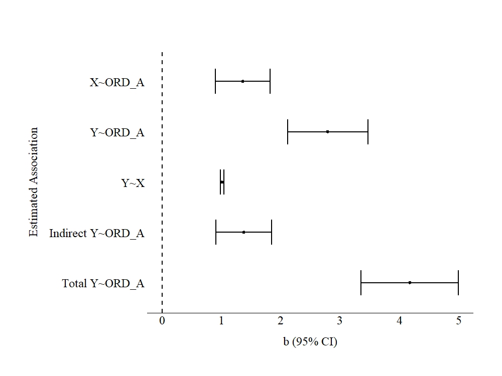
Similar to the dichotomous indicator, the ordered indicator of A was subjected to a model identical to the true model. The unstandardized effects are presented in Figure 5. The results of the model suggested that a 1-point increase on ORD_A (with a maximum of a 4-point increase) directly results in a 1.363 increase in X and a 2.793 increase in Y. Moreover, the model estimates suggest that a 1-point increase on ORD_A was indirectly associated with a 1.381 increase in Y and a total effect of 4.174.
Overall, if we were to interpret these estimates using the substantive labels, we would suggest that changes from one category to the next category of depressive symptoms results in approximately 1 more day using substances and 3 to 4 more weeks unemployed. Considering the nature of the categories, these estimates could be used to suggest that changes in the frequency and severity of experiencing symptoms of depression is associated with increased substance use and increased unemployment. While our interpretations of ordinal constructs commonly emulate those of continuous constructs, it is important to note that the interpretations of ordinal constructs should be conditional upon the scoring of the construct. Importantly, coinciding with the dichotomous model, the interpretation of the estimates associated with ORD_A provide a moderate degree of support for the development of an intervention for individuals experiencing 5 days of one symptom over the course of a year, but a high degree of support for the development of an intervention to reduce the likelihood of individuals experiencing two days of every symptom over the course of a year.
[Figure 5]
5.4. Aggregate Scale
To continue our exploration of measurement creation, let’s conceptualize A as an aggregate scale – i.e., continuous construct – and replicate the analyses. An aggregate scale can be defined as the total number of occurrences or events that each case has been exposed to. To simplify, aggregate measures represent the sum of values across multiple items. Corresponding with this, the social behavioral literature frequently uses aggregate scales when conceptualizing a wide variety of constructs. For instance, it is common in the criminal justice literature to conceptualize criminal behavior – or criminality – as the total number of crimes an individual has committed within a predefined time period. In this sense, the total number of crimes represents the raw sum of involvement in criminal activity. Similarly, psychologists frequently conceptualize the symptoms of a mental health affliction using aggregate scales. One common example is the number of days an individual experienced symptoms associated with a psychological affliction. In addition to criminologists and psychologists, behavioral scientists commonly conceptualize alcohol and drug use as the number of drinks – or drugs – an individual has within a specified time period.
For the current example, we will conceptualize A as the total number of times a case experienced symptoms associated with severe depression. To operationalize this measure, we can sum the values across Items 1-10 using the rowSums function in R. Notably, Items 1-10 capture experiencing symptoms of severe depression on a daily scale, meaning that our interpretations of the estimates must account for the aggregate scale across the original items. As demonstrated in the summary of Agg_A, the aggregate number of times a case experienced symptoms of severe depression ranged from 9-times to 3650 times.
> ## Aggregate Measure Creation ####
>
> DF$Agg_A<-rowSums(data.frame(DF$Item1,DF$Item2,DF$Item3,DF$Item4,DF$Item5,
+           DF$Item6,DF$Item7,DF$Item8,DF$Item9,DF$Item10))
>
> summary(DF$Agg_A)
         Min.       1st Qu.        Median          Mean       3rd Qu.          Max.
   9.05615663   21.52056586   25.61471561   27.10848388   30.45485381 3650.00000000
>
> ## Aggregate Model ####
>
> F1<-'
+ X~a*Agg_A
+ Y~b*Agg_A+c*X
+
+ # Indirect Effects
+ ac:=(a*c)
+ # Total Effects
+ abc:=b+(a*c)
+
+ '
>
> M1<-sem(F1,data=DF, estimator = "ML")
> SM1<-summary(M1, fit.measures= TRUE, standardized = TRUE, ci = TRUE, rsquare = T)
>
The results of the model regressing X on Agg_A and Y on Agg_A and X produced estimates suggesting that a 1-point increase in Agg_A was associated with a .012 increase in X and a .033 increase in Y. The indirect effect of Agg_A on Y suggested that a 1-point increase in Agg_A was associated with a .012 increase in Y through X, with Agg_A having a total effect on Y of .045.
To interpret these estimates with a substantive lens, the results suggest that increases in the aggregate number of days an individual experienced across the 10 symptoms of severe depression was associated with nominal changes in substance use and nominal changes in the number of weeks unemployed. Nonetheless, these estimates do suggest that an intervention would have the highest return for individuals that experienced a high aggregate number of days of symptoms but might have limited impact for individuals that experienced a low aggregate number of days symptoms.
[Figure 6]

5.5. Variety Score
Finally, let’s talk about the creation of variety scores. Variety scores are semi-continuous indicators of the number of different types of a construct an individual experienced. For example, our conceptualization of A for a variety score would be “the number of different types of symptoms of severe depression a case experienced during the past year.” In this sense, a variety score represents if an individual had a variety of different experiences or diversity in their experiences. Higher scores on variety scores commonly represent more diversity in one’s experiences, while lower scores represent less diversity in one’s experiences. Similar to the other demonstrations, a variety score has a conceptualization and operationalization distinct from dichotomous, ordered, and aggregate constructs. Variety scores are commonly used to measure constructs where diversity in experiences or exposure matters. For example, the frequency and variety of adverse childhood experiences (ACEs) can be operationalized simultaneously, providing the ability to estimate the effects of exposure and diversity in exposure to ACEs. Similarly, a variety score provides the ability to examine how diversity in victimization experiences influences outcomes of interest. Importantly, due to the distinct conceptualizations, measures that tap the frequency of exposure and the variety of exposure can be introduced into the same general linear model when examining the effects of an independent variable on a dependent variable.
For the current example, as stated above, we will conceptualize A as the number of different types of symptoms of severe depression a case experienced during the past year. To operationalize this measure, we can create dichotomies of Items 1-10, where a value of “1” indicates that a case experienced the specified symptom and a value of “0” indicates that a case did not experience the specified symptom. After creating the dichotomies for Items 1-10 (DI_Items 1-10 in the code), we can sum across the dichotomies. The resulting column (Var_A) ranges in values from 0-10 indicative of the diversity in symptoms an individual experienced during the past year.
> ## Variety Measure Creation ####
> DF$DI_Item1<-0
> DF$DI_Item2<-0
> DF$DI_Item3<-0
> DF$DI_Item4<-0
> DF$DI_Item5<-0
> DF$DI_Item6<-0
> DF$DI_Item7<-0
> DF$DI_Item8<-0
> DF$DI_Item9<-0
> DF$DI_Item10<-0
>
> DF$DI_Item1[DF$Item1>=1]<-1
> DF$DI_Item2[DF$Item2>=1]<-1
> DF$DI_Item3[DF$Item3>=1]<-1
> DF$DI_Item4[DF$Item4>=1]<-1
> DF$DI_Item5[DF$Item5>=1]<-1
> DF$DI_Item6[DF$Item6>=1]<-1
> DF$DI_Item7[DF$Item7>=1]<-1
> DF$DI_Item8[DF$Item8>=1]<-1
> DF$DI_Item9[DF$Item9>=1]<-1
> DF$DI_Item10[DF$Item10>=1]<-1
>
> DF$Var_A<-rowSums(data.frame(DF$DI_Item1,DF$DI_Item2,DF$DI_Item3,DF$DI_Item4,DF$DI_Item5,
+                              DF$DI_Item6,DF$DI_Item7,DF$DI_Item8,DF$DI_Item9,DF$DI_Item10))
>
> summary(DF$Var_A)
   Min. 1st Qu.  Median    Mean 3rd Qu.    Max.
 2.0000  7.0000  8.0000  8.1962  9.0000 10.0000

> > F1<-'
+ X~a*Var_A
+ Y~b*Var_A+c*X
+
+ # Indirect Effects
+ ac:=(a*c)
+ # Total Effects
+ abc:=b+(a*c)
+
+ '
>
> M1<-sem(F1,data=DF, estimator = "ML")
> SM1<-summary(M1, fit.measures= TRUE, standardized = TRUE, ci = TRUE, rsquare = T)
>
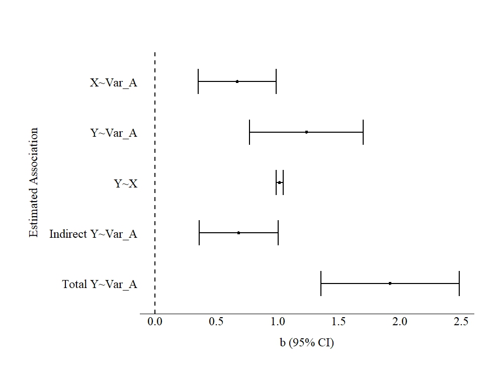
The results of the model regressing X on Var_A and Y on Var_A and X produced estimates suggesting that a 1-point increase in Var_A was associated with a .671 increase in X and a 1.236 increase in Y. The indirect effect of Var_A on Y suggested that a 1-point increase in Var_A was associated with a .682 increase in Y through X, with Var_A having a total effect on Y of 1.918.
To interpret these estimates with the substantive labels, the results suggest that increases in the number of different symptoms an individual experienced was associated with approximately a 1 day increase in substance use and a 2 week increase in unemployment. The estimated effects suggest that we should develop interventions for individuals that experience a greater diversity in depressive symptoms. That is, interventions that limited the different types of symptoms of severe depression that individuals experience could be effective at reducing these negative outcomes.
[Figure 6]
Supplemental Model
For the sake of demonstration, and because it is informative, a supplemental model was estimated where X was regressed on Var_A and Agg_A and Y on Var_A, Agg_A, and X. The results of the model (presented below) suggested that after accounting for the diversity in depressive symptoms an individual experienced (Var_A), the frequency of depressive symptoms (Agg_A) had limited impact on substance use (X). Nevertheless, Var_A, Agg_A, and X all had independent and substantively meaningful effects on Y (weeks unemployed). Moreover, the two constructs covaried to a high degree, but the effects of Var_A and Agg_A on X and Y were not substantively influenced by this covariance.
> # Supplemental Model ####
> F1<-'
+ X~a*Var_A+Agg_A
+ Y~b*Var_A+Agg_A+c*X
+
+ Agg_A~~Var_A
+
+ # Indirect Effects
+ ac:=(a*c)
+ # Total Effects
+ abc:=b+(a*c)
+
+ '
>
> M1<-sem(F1,data=DF, estimator = "ML")
> summary(M1, fit.measures= TRUE, standardized = TRUE, ci = TRUE, rsquare = T)
lavaan 0.6-12 ended normally after 8 iterations

Regressions:
                   Estimate  Std.Err  z-value  P(>|z|) ci.lower ci.upper   Std.lv  Std.all
  X ~
    Var_A      (a)    0.637    0.163    3.910    0.000    0.318    0.956    0.637    0.039
    Agg_A             0.009    0.006    1.670    0.095   -0.002    0.020    0.009    0.017
  Y ~
    Var_A      (b)    1.133    0.238    4.752    0.000    0.666    1.600    1.133    0.039
    Agg_A             0.028    0.008    3.528    0.000    0.013    0.044    0.028    0.029
    X          (c)    1.016    0.015   69.490    0.000    0.987    1.045    1.016    0.570

Covariances:
                   Estimate  Std.Err  z-value  P(>|z|) ci.lower ci.upper   Std.lv  Std.all
  Var_A ~~
    Agg_A             5.761    0.471   12.238    0.000    4.838    6.683    5.761    0.123

Variances:
                   Estimate  Std.Err  z-value  P(>|z|) ci.lower ci.upper   Std.lv  Std.all
   .X               413.365    5.846   70.711    0.000  401.908  424.823  413.365    0.998
   .Y               883.723   12.498   70.711    0.000  859.228  908.218  883.723    0.670
    Var_A             1.582    0.022   70.711    0.000    1.538    1.625    1.582    1.000
    Agg_A          1380.131   19.518   70.711    0.000 1341.876 1418.386 1380.131    1.000

R-Square:
                   Estimate
    X                 0.002
    Y                 0.330

Defined Parameters:
                   Estimate  Std.Err  z-value  P(>|z|) ci.lower ci.upper   Std.lv  Std.all
    ac                0.647    0.166    3.904    0.000    0.322    0.972    0.647    0.022
    abc               1.780    0.290    6.137    0.000    1.211    2.349    1.780    0.062

>
6. Discussion and Conclusion
The current entry has reviewed measurement creation and the effects of different operationalizations on the associations between A and X and A and Y. As demonstrated above, none of the operationalizations of A using Items 1-10 replicated the estimates produced in the true model (i.e., the model estimated when treating A as observed). Specifically, some of our findings suggested that the magnitude of the association between A and X and A and Y was stronger than reality, while some of our findings suggested that the magnitude of the association was weaker than reality. Nevertheless, it is important to note that each operationalization required a different conceptualization of A, highlighting one of the sources of statistical bias in measurement creation. That is, if one clearly defines what A represents and properly operationalizes A, the differences between the estimated effects of A on X and A on Y across the models can be expected. Nevertheless, similar to previous entries, statistical bias associated with measurement often corresponds with the implementation of an operationalization that does not accurately quantify the conceptualized construct. If this source of statistical bias exists within your model, the interpretations, conclusions, and policy implications associated with the model will become biased.
In addition to highlighting the importance of properly conceptualizing and operationalizing a construct, the current entry served to demonstrate the effects of measurement error in observed items. Although the magnitude of the influence of measurement error on the model estimates was not clearly demonstrated, the estimated effects produced by the models were influenced by the existence of measurement error in Items 1-10. This can be observed by reviewing the standardized slope coefficients and R-squared values produced by the statistical models (available in the R-code). Evident by the standardized slope coefficients and R-squared values, the variation explained in X and Y varies across the measures of A, which was also distinct from the variation in X and Y explained by A when A was treated as an observed construct (i.e., the true model). Overall, this entry provides two important messages: 1) make sure your operationalization of a construct matches the conceptualization of the construct and 2) consider the potential effects of measurement error when operationalizing a construct of interest.
[i] To briefly reiterate, this bias exists because general linear models rely on the covariance matrix when estimating the effects of one construct on another construct independent of observed confounders.
[ii] Note, I did not define the concept of income because multiple definitions exist. For instance, the concept of income can be defined as gross earnings, net earnings, earnings from legal employment, earnings from legal and illegal employment, etc.
