1. Introduction (PDF & R-Script)
The prior entries in the current section reviewed the impact of altering the level of measurement of the dependent variable (Entry 13) and independent variable (Entry 14) on the magnitude of the estimated association. These entries demonstrated that the level of measurement reduced the magnitude of the estimated association between independent and dependent variable – demonstrated using the hypothesis testing statistics. Specifically, the simulations illustrated that the employment of a continuous coding scheme for both the independent and dependent variable produced estimates demonstrating the strongest statistical association, while a dichotomous coding scheme produced estimates demonstrating the weakest statistical association. Overall, altering the operationalization of the dependent variable and the independent variable impacts the estimated association. In practice, however, the dependent variable and the independent variable will likely be operationalized in a manner that maximizes the information captured across the population. As such, it can be argued that while the operationalization of the constructs of interest is important, the operationalization of covariates we introduce into multivariable models could be more important!
We tend to care less about maximizing the information captured by covariates included in our statistical models. And, on some occasions, scholars are outright encouraged to simplify multivariable models by only including dichotomous covariates.[i] To provide an example in the literature, it is common for scholars in sociology, psychology, and criminology to adjust for an individual’s level of educational attainment when estimating the effects of an independent variable on a dependent variable. There are multiple ways to operationalize educational attainment – e.g., years of schooling (continuous) or highest degree earned (ordinal) –, of which the dichotomous operationalization of Completed High School (“1” = Yes) or Completed College (“1” = Yes) are commonly included in multivariable models. As it is often perceived, including either Completed High School or Completed College in a multivariable model adjusts for the confounding effects of educational attainment on the association being estimated (for example, when estimating the effects of criminal behavior on employment). Although beneficial if educational attainment does confound the association, operationalizing educational attainment as a dichotomous construct (e.g., completed high school) limits the amount of variation adjusted for when including the covariate in a multivariable model. In this sense, the estimated association between the independent and dependent variable will vary – or become biased – conditional upon the level of measurement of the confounder.[ii]
Similarly, the bias associated with the inclusion of a collider in a statistical model will vary conditional upon the operationalization of a collider. For example, opposite of a confounder, operationalizing a collider as an ordinal or dichotomous construct– when compared to a continuous construct – can reduce the amount of bias observed when estimating the association between the independent and dependent variable of interest. On an analogous note, the level of measurement of a mediator when included as covariates influences the estimates corresponding to the direct effects of the independent variable on the dependent variable, while the level of measurement of a moderator influences the estimates corresponding to an interaction effect. For instance, including a mediator measured dichotomously in a multivariable model will produce estimates for the direct effects of the independent variable on the dependent variable distinct from the estimates produced if the mediator was measured ordinally.
More broadly, operationalizing a covariate as a continuous construct adjusts for the maximum amount of variation shared between the covariate, independent variable, and dependent variable. However, when the covariate is operationalized using an ordered scale – or as a dichotomy – the amount of shared variation adjusted for through the estimation of a multivariable model is reduced. The reduction in the shared variation, in turn impacts the estimates produced by the multivariable model. And, in particular, can introduce – or reduce – bias when estimating the association between the covariate and the dependent variable, as well as when estimating the association between the independent variable and the dependent variable. As demonstrated in the simulations below, these biases can substantively alter our interpretation of the association between the independent and dependent variable of interest.
2. Confounder
To briefly review, a confounder is a construct that causes variation in both the independent and dependent variable. Not adjusting for a confounder in a statistical model will result in a biased estimate of the effects of the independent variable on the dependent variable. The direction and magnitude of that bias, however, is conditional upon the direction and magnitude of the causal effects of the confounder on the independent variable and the dependent variable. Entry 7 provides a detailed review of confounder bias.
To begin our simulation, we first must specify the confounder (“Con” in the R-code). 10,000 scores for Con were drawn from a normal distribution with a mean of 0 and a standard deviation of 10. After simulating a vector of scores to represent the confounder, scores on X were specified to be causally influenced by scores on Con plus a random value drawn from a normal distribution with a mean of 0 and a standard deviation of 10. Concerning the dependent variable, scores on Y were specified to be causally influenced by scores on X and scores on Con plus a random value drawn from a normal distribution with a mean of 0 and a standard deviation of 30. Using the specification below, a 1-point increase in X was specified to cause a 1-point increase in Y, while a 1-point increase in Con was specified to cause a 4-point increase in Y. A 1-point increase in Con was also specified to cause a 4-point increase in X.
To ensure that the simulation specification produced a confounded association between X and Y, a bivariate linear regression model was estimated. Evident by the findings, the estimates suggested that a 1-point increase in X corresponded to approximately a 2-point increase in Y, highlighting that our model needs to adjust for the variation in Con to produce an estimate representative of the true causal association between X and Y (i.e., b = 1).
> # Confounders ####
> n<-10000
>
> set.seed(1992)
>
> Con<-1*rnorm(n,0,10)
> X<-1*rnorm(n,0,10)+4*Con
> Y<-1*X+1*rnorm(n,0,30)+4*Con
>
> DF<-data.frame(Con,X,Y)
>
> M1<-glm(Y~X, data = DF, family = gaussian(link = "identity"))
> summary(M1)

Call:
glm(formula = Y ~ X, family = gaussian(link = "identity"), data = DF)

Deviance Residuals:
     Min        1Q    Median        3Q       Max
-109.617   -21.412     0.056    21.120   117.419

Coefficients:
             Estimate Std. Error t value Pr(>|t|)
(Intercept) -0.663385   0.312699  -2.121   0.0339 *
X            1.929342   0.007549 255.559   <2e-16 ***
---
Signif. codes:  0 ‘***’ 0.001 ‘**’ 0.01 ‘*’ 0.05 ‘.’ 0.1 ‘ ’ 1

(Dispersion parameter for gaussian family taken to be 977.681)

    Null deviance: 73627829  on 9999  degrees of freedom
Residual deviance:  9774855  on 9998  degrees of freedom
AIC: 97235

Number of Fisher Scoring iterations: 2

>
2.1. Continuous Confounder
Now let’s estimate a multivariable model adjusting for the variation in Con. In the model presented below, Con is coded as a continuous construct. Adjusting for the variation in Con, evident by the results, permits us to produce an estimate representative of the true causal association between X and Y. In particular, the slope of the association between X and Y when adjusting for Con is .971, which is substantively identical to the true causal association between X and Y (1.00). The similarity between the estimated association and the specified association is further highlighted in Figure 1, where the estimated linear regression line is visually identical to a slope of 1.00.
> ## Adjusting for Continuous Confounder ####
>
> M2<-glm(Y~X+Con, data = DF, family = gaussian(link = "identity"))
> summary(M2)

Call:
glm(formula = Y ~ X + Con, family = gaussian(link = "identity"),
    data = DF)

Deviance Residuals:
     Min        1Q    Median        3Q       Max
-110.923   -19.962     0.249    20.273   126.040

Coefficients:
            Estimate Std. Error t value Pr(>|t|)
(Intercept) -0.76368    0.29672  -2.574   0.0101 *
X            0.97098    0.02967  32.729   <2e-16 ***
Con          4.08914    0.12284  33.289   <2e-16 ***
---
Signif. codes:  0 ‘***’ 0.001 ‘**’ 0.01 ‘*’ 0.05 ‘.’ 0.1 ‘ ’ 1

(Dispersion parameter for gaussian family taken to be 880.2107)

    Null deviance: 73627829  on 9999  degrees of freedom
Residual deviance:  8799466  on 9997  degrees of freedom
AIC: 96185

Number of Fisher Scoring iterations: 2

>
2.2. Ordered Confounder
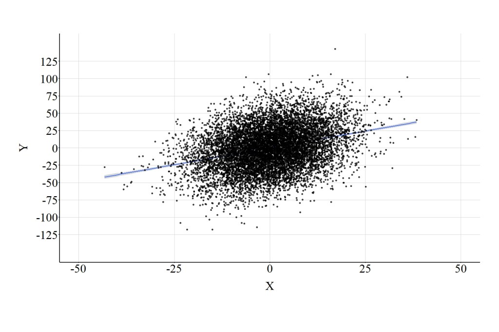
Now let’s recode Con as an ordered construct and include it as a covariate in a multivariable model. To recode Con, we can split the distribution at the quartiles. That is, cases that initially scored between 0 and the 25th percentile received a value of “1”, cases that scored between the 25th and the 50th percentile received a value of “2”, cases that scored between the 50th and the 75th percentile received a value of “3”, and cases that scored between the 75th and the 100th percentile received a value of “4.” This coding scheme generated a distribution where an equal number of cases – 2,500 – received a 1, 2, 3, or 4. This measure was re-labeled as Con_OR1, and included as a covariate when regressing Y on X. The results of the regression model adjusting for Con_OR1 are presented below. Focusing on the association between X and Y, the estimated slope coefficient was 1.686 suggesting that a 1-point increase in X corresponded to a 1.686-point increase in Y. Substantively, the estimates for the association between X and Y when adjusting for Con_OR1 are distinct from the estimates produced by the model adjusting for the continuous version of Con. In particular, adjusting for Con_OR1 produced a slope coefficient closer to the confounded slope coefficient (b = 1.929) than the unconfounded slope coefficient (b = .971). The distinction between adjusting for the continuous version of Con and the ordered version of Con is further highlighted by Figure 2 (pay close attention to the scale of the X and Y axes).
> ## Adjusting for Ordered Confounder ####
>
> summary(DF$Con)
    Min.  1st Qu.   Median     Mean  3rd Qu.     Max.
-39.0733  -6.6657   0.0075   0.1341   6.9267  39.3637
> DF$Con_OR1<-NA
> DF$Con_OR1[DF$Con>=quantile(DF$Con,0) & DF$Con < quantile(DF$Con,.25)]<-1
> DF$Con_OR1[DF$Con>=quantile(DF$Con,.25) & DF$Con < quantile(DF$Con,.50)]<-2
> DF$Con_OR1[DF$Con>=quantile(DF$Con,.50) & DF$Con < quantile(DF$Con,.75)]<-3
> DF$Con_OR1[DF$Con>=quantile(DF$Con,.75) & DF$Con <= quantile(DF$Con,1)]<-4
> summary(DF$Con_OR1)
   Min. 1st Qu.  Median    Mean 3rd Qu.    Max.
   1.00    1.75    2.50    2.50    3.25    4.00
> table(DF$Con_OR1)

   1    2    3    4
2500 2500 2500 2500
>
> M2<-glm(Y~X+Con_OR1, data = DF, family = gaussian(link = "identity"))
> summary(M2)

Call:
glm(formula = Y ~ X + Con_OR1, family = gaussian(link = "identity"),
    data = DF)

Deviance Residuals:
     Min        1Q    Median        3Q       Max
-107.874   -21.115     0.107    20.940   114.571

Coefficients:
            Estimate Std. Error t value Pr(>|t|)
(Intercept) -25.6402     1.5888  -16.14   <2e-16 ***
X             1.6862     0.0169   99.75   <2e-16 ***
Con_OR1      10.0362     0.6262   16.03   <2e-16 ***
---
Signif. codes:  0 ‘***’ 0.001 ‘**’ 0.01 ‘*’ 0.05 ‘.’ 0.1 ‘ ’ 1

(Dispersion parameter for gaussian family taken to be 953.2869)

    Null deviance: 73627829  on 9999  degrees of freedom
Residual deviance:  9530009  on 9997  degrees of freedom
AIC: 96983

Number of Fisher Scoring iterations: 2

>

2.3. Dichotomous Confounder
Following the trend, now let’s dichotomize Con by splitting the distribution at the median. Specifically, cases with a score on Con equal to or below the mediate received a score of “0” on Con_DI1, while cases with a score on Con greater than the median received a score “1” on Con_DI1. Including this as a covariate in the model produced estimates almost identical to the confounder regression model (i.e., the bivariate linear regression model of X on Y). Specifically, the estimated association suggests that a 1-point change in X corresponded to a 1.842-point change in Y after adjusting for the variation in Con_DI1. Of particular interest, these findings suggest that adjusting for Con_DI1 does not appear to produce estimates substantively distinct from the estimates produced when we did not adjust for the variation in Con. This interpretation is further supported by Figure 3.
> ## Adjusting for Dichotomous Confounder ####
>
> summary(DF$Con)
    Min.  1st Qu.   Median     Mean  3rd Qu.     Max.
-39.0733  -6.6657   0.0075   0.1341   6.9267  39.3637
> DF$Con_DI1<-NA
> DF$Con_DI1[DF$Con<=median(DF$Con)]<-0
> DF$Con_DI1[DF$Con>median(DF$Con)]<-1
> summary(DF$Con_DI1)
   Min. 1st Qu.  Median    Mean 3rd Qu.    Max.
    0.0     0.0     0.5     0.5     1.0     1.0
> table(DF$Con_DI1)

   0    1
5000 5000
>
> M2<-glm(Y~X+Con_DI1, data = DF, family = gaussian(link = "identity"))
> summary(M2)

Call:
glm(formula = Y ~ X + Con_DI1, family = gaussian(link = "identity"),
    data = DF)

Deviance Residuals:
    Min       1Q   Median       3Q      Max
-109.69   -21.22     0.26    21.11   117.15

Coefficients:
            Estimate Std. Error t value Pr(>|t|)
(Intercept) -5.25427    0.58067  -9.049   <2e-16 ***
X            1.84246    0.01194 154.323   <2e-16 ***
Con_DI1      9.26304    0.98896   9.366   <2e-16 ***
---
Signif. codes:  0 ‘***’ 0.001 ‘**’ 0.01 ‘*’ 0.05 ‘.’ 0.1 ‘ ’ 1

(Dispersion parameter for gaussian family taken to be 969.2729)

    Null deviance: 73627829  on 9999  degrees of freedom
Residual deviance:  9689821  on 9997  degrees of freedom
AIC: 97149

Number of Fisher Scoring iterations: 2

>
2.4. Summary of Results
As demonstrated, the estimated effects of X on Y produced by the multivariable model varied conditional upon the level of measurement for the confounder. When measured continuously, adjusting for the confounder in a multivariable model produced estimates for the association between X and Y that emulated the specification of the simulated data. When measured ordinally, adjusting for the confounder in a multivariable model produced estimates for the association between X and Y closer to the bivariate model than the model adjusting for the continuous version of the confounder. When measured dichotomously, adjusting for the confounder in a multivariable model produced estimates for the association between X and Y extremely similar to the bivariate model. Overall, when a construct is postulated to confound an association of interest, operationalizing the construct continuously and including it as a covariate in a multivariable model will provide the best opportunity – when compared to an ordered or dichotomous operationalization – to observe the causal association between the variables of interest.
3. Collider
Collider variables exist when two or more constructs cause variation in a single construct. In this simulation, our independent and dependent variables (X and Y) will be specified to cause variation in a single construct (Col) and generate a collision. Distinct from a confounder, the inclusion of a collider in a multivariable model will result in the estimation of a biased association between the independent variable and the dependent variable (Reviewed in Entry 8). The direction and magnitude of the bias is conditional upon the direction and magnitude of the causal influence of the independent variable and the dependent variable on the collider.
To simulate a collision, or a collider variable, we first simulate scores drawn from a normal distribution with a mean of 0 and a standard deviation of 10 to represent our independent variable (X). After which, we specify that scores on Y are causally influenced by scores on X – where a 1-point increase in X corresponds to a 1-point increase in Y – plus a random value drawn from a normal distribution with a mean of 0 and a standard deviation of 30. Finally, we simulate the collider (Col) by specifying that scores are causally influenced by X and Y, plus a value randomly drawn from a normal distribution with a mean of 0 and a standard deviation of 10. In this simulation, a 1-point increase in X or Y was specified to result in a 4-point increase in the collider.
To begin our analysis, let’s estimate the bivariate association between X and Y. The results of the model – presented below – emulated the simulation specification, producing evidence that a 1-point increase in X corresponded to a 1.054-point increase in Y. The difference (∆b = .054) corresponds to the random variation specified to exist in X and Y. Importantly, in this simulation, association between X and Y will only become biased when Col is included as a covariate in the regression equation. So, let’s do that.
> # Colliders ####
> n<-10000
>
> set.seed(1992)
>
>
> X<-1*rnorm(n,0,10)
> Y<-1*X+1*rnorm(n,0,30)
> Col<-1*rnorm(n,0,10)+ 4*X+4*Y
>
> DF<-data.frame(Col,X,Y)
>
> M1<-glm(Y~X, data = DF, family = gaussian(link = "identity"))
> summary(M1)

Call:
glm(formula = Y ~ X, family = gaussian(link = "identity"), data = DF)

Deviance Residuals:
     Min        1Q    Median        3Q       Max
-129.757   -20.018     0.071    20.265   115.132

Coefficients:
            Estimate Std. Error t value Pr(>|t|)
(Intercept)  -0.2138     0.3001  -0.713    0.476
X             1.0541     0.0300  35.143   <2e-16 ***
---
Signif. codes:  0 ‘***’ 0.001 ‘**’ 0.01 ‘*’ 0.05 ‘.’ 0.1 ‘ ’ 1

(Dispersion parameter for gaussian family taken to be 900.2438)

    Null deviance: 10112469  on 9999  degrees of freedom
Residual deviance:  9000637  on 9998  degrees of freedom
AIC: 96409

Number of Fisher Scoring iterations: 2

>
3.1. Continuous Collider
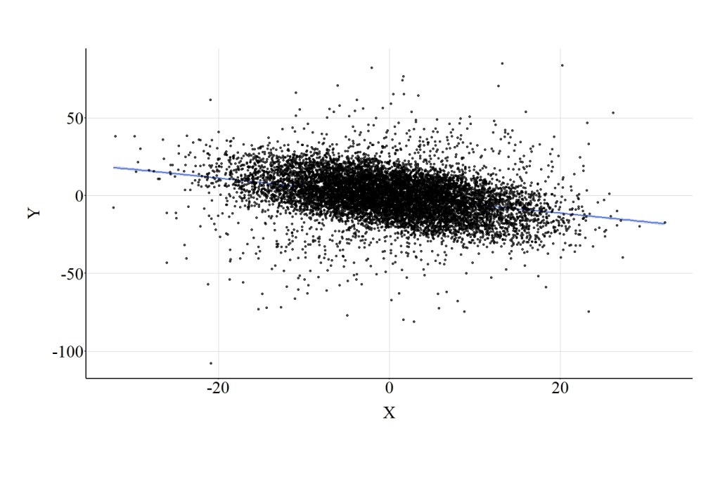
Here, we estimate a multivariable regression model evaluating the effects of X on Y adjusting for the variation in Col. The estimates of this regression model suggest that X has a negative influence on Y, where a 1-point increase in X corresponds to a -.985 reduction in Y. This substantive departure from the bivariate association is observed because Col was included in the model as a covariate, highlighting the effects of collider bias on the interpretation corresponding to the association of interest. Figure 4 highlights the negative association between X and Y that is observed when the multivariable model adjusts for Col.
> ## Adjusting for Continuous Collider ####
>
> M2<-glm(Y~X+Col, data = DF, family = gaussian(link = "identity"))
> summary(M2)

Call:
glm(formula = Y ~ X + Col, family = gaussian(link = "identity"),
    data = DF)

Deviance Residuals:
     Min        1Q    Median        3Q       Max
-10.0943   -1.6864   -0.0158    1.6730    9.1198

Coefficients:
             Estimate Std. Error  t value Pr(>|t|)
(Intercept)  0.061816   0.024663    2.506   0.0122 *
X           -0.985497   0.002985 -330.201   <2e-16 ***
Col          0.248512   0.000205 1212.479   <2e-16 ***
---
Signif. codes:  0 ‘***’ 0.001 ‘**’ 0.01 ‘*’ 0.05 ‘.’ 0.1 ‘ ’ 1

(Dispersion parameter for gaussian family taken to be 6.081088)

    Null deviance: 10112469  on 9999  degrees of freedom
Residual deviance:    60793  on 9997  degrees of freedom
AIC: 46436

Number of Fisher Scoring iterations: 2

>
3.2. Ordered Collider
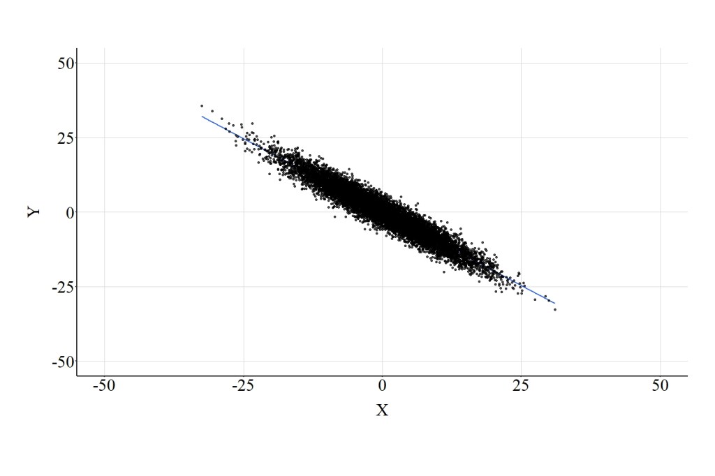
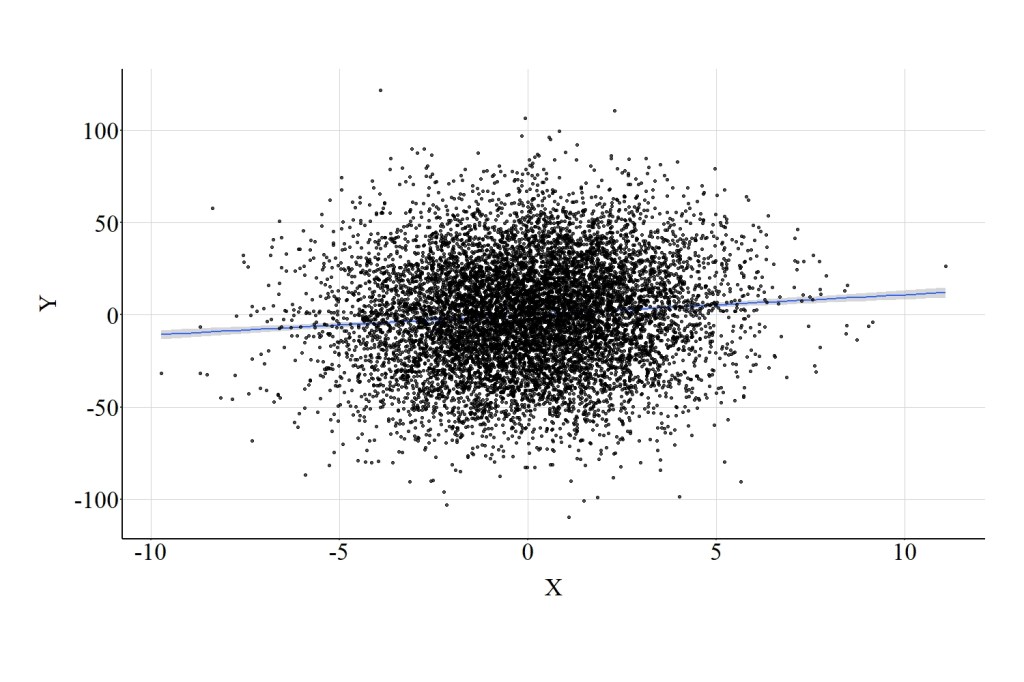
Now let’s recode Col into an ordinal variable. Here, following the steps discussed when recoding Con to Con_OR1, we can create Col_OR1. The cases received a 1, 2, 3, or 4 on Col_OR1 conditional upon their ranked position in the Col distribution. While the estimated effects of X on Y remained negative when adjusting for Col_OR1, the slope coefficient became attenuated (closer to zero) when compared to the model adjusting for the continuous version of Col. Specifically, the results of this model suggest that a 1-point increase in X corresponded to a .563 reduction in Y. Figure 5 further highlights the negative association between X and Y that is observed when the multivariable model adjusts for Col_OR1, while also illustrating the distinct effects of the continuous and ordered versions of Col when estimating the association between X and Y.
> ## Adjusting for Ordered Collider ####
>
> summary(DF$Col)
     Min.   1st Qu.    Median      Mean   3rd Qu.      Max.
-693.6215  -97.7149    1.2271   -0.0083   98.2333  608.0042
> DF$Col_OR1<-NA
> DF$Col_OR1[DF$Col>=quantile(DF$Col,0) & DF$Col < quantile(DF$Col,.25)]<-1
> DF$Col_OR1[DF$Col>=quantile(DF$Col,.25) & DF$Col < quantile(DF$Col,.50)]<-2
> DF$Col_OR1[DF$Col>=quantile(DF$Col,.50) & DF$Col < quantile(DF$Col,.75)]<-3
> DF$Col_OR1[DF$Col>=quantile(DF$Col,.75) & DF$Col <= quantile(DF$Col,1)]<-4
> summary(DF$Col_OR1)
   Min. 1st Qu.  Median    Mean 3rd Qu.    Max.
   1.00    1.75    2.50    2.50    3.25    4.00
> table(DF$Col_OR1)

   1    2    3    4
2500 2500 2500 2500
>
> M2<-glm(Y~X+Col_OR1, data = DF, family = gaussian(link = "identity"))
> summary(M2)

Call:
glm(formula = Y ~ X + Col_OR1, family = gaussian(link = "identity"),
    data = DF)

Deviance Residuals:
     Min        1Q    Median        3Q       Max
-119.692    -8.028     0.146     8.188    95.315

Coefficients:
             Estimate Std. Error t value Pr(>|t|)
(Intercept) -69.74158    0.38373 -181.74   <2e-16 ***
X            -0.56283    0.01607  -35.03   <2e-16 ***
Col_OR1      27.89785    0.14376  194.06   <2e-16 ***
---
Signif. codes:  0 ‘***’ 0.001 ‘**’ 0.01 ‘*’ 0.05 ‘.’ 0.1 ‘ ’ 1

(Dispersion parameter for gaussian family taken to be 188.8634)

    Null deviance: 10112469  on 9999  degrees of freedom
Residual deviance:  1888068  on 9997  degrees of freedom
AIC: 80794

Number of Fisher Scoring iterations: 2

>
3.3. Dichotomous Collider
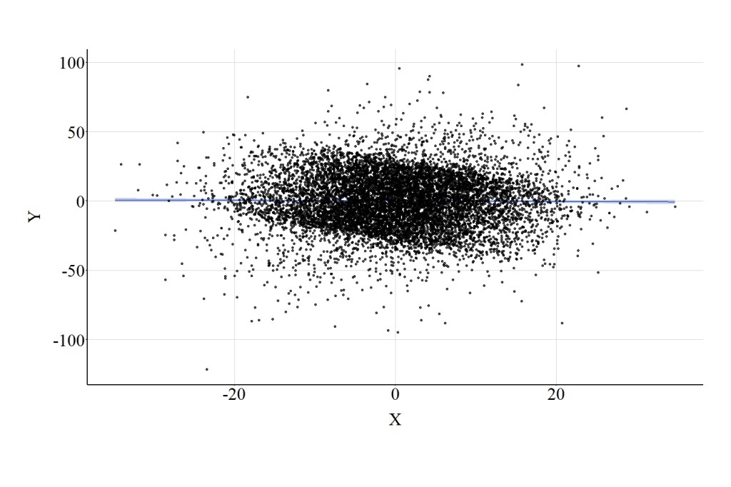
Similar to the confounder demonstration, let’s recode our collider into a dichotomous construct and introduce it into our multivariable model. Cases that scored below or equal to the median of Col received a “0” on Col_DI1, while cases that scored above the median received a “1” on Col_DI1. When adjusting for Col_DI1, the results of the multivariable regression model suggested that a 1-point increase in X corresponded to a .02-point reduction in Y. The magnitude of this point estimate is extremely close to zero, suggesting that the variation in X does not predict the variation in Y when adjusting for Col_DI1. The interpretation associated with these estimates is distinct from the preceding models, which suggested that X has a notable negative influence on Y. The horizontal regression line presented in Figure 6 further highlights the distinction between the estimates produced by the model below and the estimates produced by the prior models.
> ## Adjusting for Dichotomous Collider ####
>
> summary(DF$Col)
     Min.   1st Qu.    Median      Mean   3rd Qu.      Max.
-693.6215  -97.7149    1.2271   -0.0083   98.2333  608.0042
> DF$Col_DI1<-NA
> DF$Col_DI1[DF$Col<=median(DF$Col)]<-0
> DF$Col_DI1[DF$Col>median(DF$Col)]<-1
> summary(DF$Col_DI1)
   Min. 1st Qu.  Median    Mean 3rd Qu.    Max.
    0.0     0.0     0.5     0.5     1.0     1.0
> table(DF$Col_DI1)

   0    1
5000 5000
>
> M2<-glm(Y~X+Col_DI1, data = DF, family = gaussian(link = "identity"))
> summary(M2)

Call:
glm(formula = Y ~ X + Col_DI1, family = gaussian(link = "identity"),
    data = DF)

Deviance Residuals:
     Min        1Q    Median        3Q       Max
-121.920   -13.379    -0.124    13.835    98.838

Coefficients:
             Estimate Std. Error t value Pr(>|t|)
(Intercept) -24.59034    0.30358 -81.001   <2e-16 ***
X            -0.02049    0.02264  -0.905    0.366
Col_DI1      49.04129    0.45302 108.254   <2e-16 ***
---
Signif. codes:  0 ‘***’ 0.001 ‘**’ 0.01 ‘*’ 0.05 ‘.’ 0.1 ‘ ’ 1

(Dispersion parameter for gaussian family taken to be 414.4736)

    Null deviance: 10112469  on 9999  degrees of freedom
Residual deviance:  4143493  on 9997  degrees of freedom
AIC: 88654

Number of Fisher Scoring iterations: 2

>
3.4. Summary of Results
The results of the three models illustrate the importance of the level of measurement for a collider when estimating an association of interest. Introducing a continuous collider into a multivariable model will increase – comparatively – the bias in the estimated association between the independent and dependent variable. Introducing a dichotomous collider into a multivariable model will decrease – comparatively – the bias in the estimated association between the independent and dependent variable. Prominently, however, it is important to consider that the level of measurement for a collider can result in distinct interpretations for the association of interest. As illustrated, including the continuous and ordinal versions of the collider in a multivariable model resulted in estimates suggesting a negative association between X and Y, while including the dichotomous version of the collider in a multivariable model resulted in estimates suggesting no association between X and Y.
4. Mediators
Mediators represent constructs where the variation is caused by the independent variable of interest, and cause variation in the dependent variable of interest. As discussed in Entry 9, the effects of X on Y can be demarcated into three categories: total effects, direct effects, and indirect effects. When a mediator does exist, the estimates produced when modeling the bivariate association between X and Y represents the total effect of X on Y. The estimates corresponding to the association between X and Y when a mediator is included as a covariate in a regression model represents the direct effect of X on Y. The indirect effects can not be illuminated unless multiple regression models or a path model is estimated. In this section, we will focus on estimating the direct effect of X on Y when adjusting for a continuous, ordered, or dichotomous mediator.
To simulate the data, we can first begin by specifying for X to be a vector of scores randomly drawn from a normal distribution with a mean of 0 and a standard deviation of 10. The Mediator (Med in the code) is specified to be causally influenced by the cases’ score on X plus a random value drawn from a normal distribution with a mean of 0 and a standard deviation of 10. A 1-point increase in X was specified to be associated with a 4-point increase in Med. Y was specified to be causally influenced by X (i.e., the direct pathway) and Med (i.e., the indirect pathway) plus a random value drawn from a normal distribution with a mean of 0 and a standard deviation of 30. The direct effects of X on Y were specified to equal 1, where a 1-point increase in X would correspond with a 1-point increase in Y, while a 1-point increase in Med was specified to cause a 4-point increase in Y.
Let’s start by estimating the total effect of X on Y using a bivariate regression model. The results of this bivariate regression model suggest that a 1-point increase in X results in a 17-point increase in Y. This estimate is correct, as the total effect of X on Y would be calculated as the multiplication of the indirect pathway plus the direct pathway, which is (4*4) + 1 ≈ 17.
> # Mediators ####
> n<-10000
>
> set.seed(1992)
>
>
> X<-1*rnorm(n,0,10)
> Med<-1*rnorm(n,0,10)+ 4*X
> Y<-1*X+4*Med+1*rnorm(n,0,30)
>
>
> DF<-data.frame(Med,X,Y)
>
> M1<-glm(Y~X, data = DF, family = gaussian(link = "identity"))
> summary(M1)

Call:
glm(formula = Y ~ X, family = gaussian(link = "identity"), data = DF)

Deviance Residuals:
     Min        1Q    Median        3Q       Max
-182.689   -33.573     0.216    32.721   209.901

Coefficients:
            Estimate Std. Error t value Pr(>|t|)
(Intercept) -1.04673    0.49577  -2.111   0.0348 *
X           17.04472    0.04956 343.932   <2e-16 ***
---
Signif. codes:  0 ‘***’ 0.001 ‘**’ 0.01 ‘*’ 0.05 ‘.’ 0.1 ‘ ’ 1

(Dispersion parameter for gaussian family taken to be 2457.418)

    Null deviance: 315255964  on 9999  degrees of freedom
Residual deviance:  24569262  on 9998  degrees of freedom
AIC: 106451

Number of Fisher Scoring iterations: 2

>
4.1. Continuous Mediator
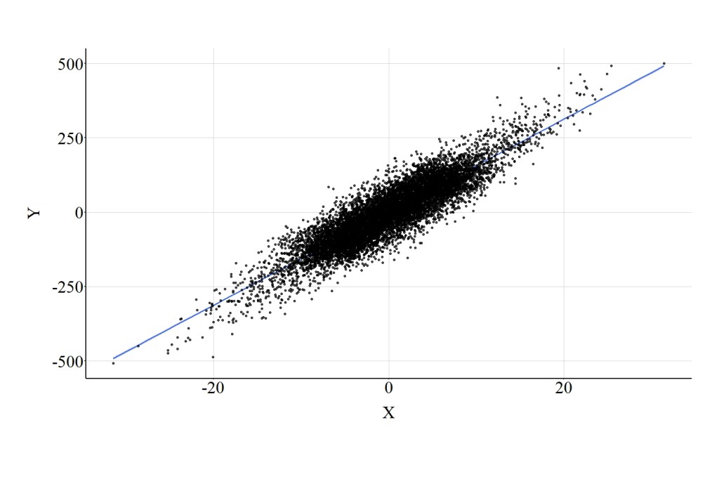
To estimate the direct effect of X on Y, we can include the continuous mediator – Med – as a covariate in the model. The results of this multivariable model suggest, consistent with the simulation specification, that a 1-point increase in X corresponds to a 1.089-point increase in Y. The direct effect of X on Y when adjusting for the continuous mediator is illustrated in Figure 7.
> ## Adjusting for Continuous Mediator ####
>
> M2<-glm(Y~X+Med, data = DF, family = gaussian(link = "identity"))
> summary(M2)

Call:
glm(formula = Y ~ X + Med, family = gaussian(link = "identity"),
    data = DF)

Deviance Residuals:
     Min        1Q    Median        3Q       Max
-110.923   -19.962     0.249    20.273   126.040

Coefficients:
            Estimate Std. Error t value Pr(>|t|)
(Intercept) -0.76368    0.29672  -2.574   0.0101 *
X            1.08914    0.12284   8.866   <2e-16 ***
Med          3.97098    0.02967 133.850   <2e-16 ***
---
Signif. codes:  0 ‘***’ 0.001 ‘**’ 0.01 ‘*’ 0.05 ‘.’ 0.1 ‘ ’ 1

(Dispersion parameter for gaussian family taken to be 880.2107)

    Null deviance: 315255964  on 9999  degrees of freedom
Residual deviance:   8799466  on 9997  degrees of freedom
AIC: 96185

Number of Fisher Scoring iterations: 2

>
4.2. Ordered Mediator
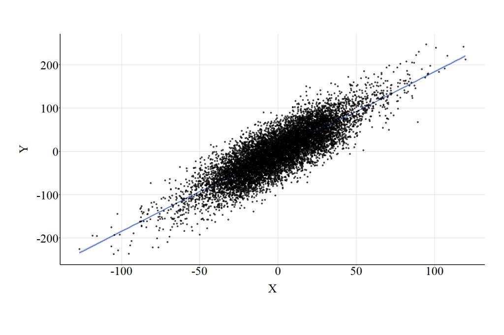
Now let’s focus on our ordered version of the mediator (Med_OR1). Med_OR1 was created using the same recoding scheme as previously discussed. When Med_OR1 was included as a covariate in the multivariable model, the magnitude of the direct effect of X on Y was estimated to be 13.007. That is, a 1-point increase in X corresponds to a 13.006-point increase in Y. Substantively, this estimate is distinct from the true direct effect (b = 1.000) and closer to the total effect of X on Y (17.000). The change in the magnitude of the estimated direct effect can be observed by comparing the regression line presented in Figure 7 to the regression line presented in Figure 8.
> ## Adjusting for Ordered Mediator ####
>
> summary(DF$Med)
     Min.   1st Qu.    Median      Mean   3rd Qu.      Max.
-158.5572  -27.8877    0.2188    0.4677   28.5786  152.4684
> DF$Med_OR1<-NA
> DF$Med_OR1[DF$Med>=quantile(DF$Med,0) & DF$Med < quantile(DF$Med,.25)]<-1
> DF$Med_OR1[DF$Med>=quantile(DF$Med,.25) & DF$Med < quantile(DF$Med,.50)]<-2
> DF$Med_OR1[DF$Med>=quantile(DF$Med,.50) & DF$Med < quantile(DF$Med,.75)]<-3
> DF$Med_OR1[DF$Med>=quantile(DF$Med,.75) & DF$Med <= quantile(DF$Med,1)]<-4
> summary(DF$Med_OR1)
   Min. 1st Qu.  Median    Mean 3rd Qu.    Max.
   1.00    1.75    2.50    2.50    3.25    4.00
> table(DF$Med_OR1)

   1    2    3    4
2500 2500 2500 2500
>
> M2<-glm(Y~X+Med_OR1, data = DF, family = gaussian(link = "identity"))
> summary(M2)

Call:
glm(formula = Y ~ X + Med_OR1, family = gaussian(link = "identity"),
    data = DF)

Deviance Residuals:
    Min       1Q   Median       3Q      Max
-204.57   -29.45    -0.24    29.63   209.92

Coefficients:
             Estimate Std. Error t value Pr(>|t|)
(Intercept) -101.0341     2.3482  -43.03   <2e-16 ***
X             13.0065     0.1036  125.60   <2e-16 ***
Med_OR1       40.2116     0.9265   43.40   <2e-16 ***
---
Signif. codes:  0 ‘***’ 0.001 ‘**’ 0.01 ‘*’ 0.05 ‘.’ 0.1 ‘ ’ 1

(Dispersion parameter for gaussian family taken to be 2067.981)

    Null deviance: 315255964  on 9999  degrees of freedom
Residual deviance:  20673608  on 9997  degrees of freedom
AIC: 104727

Number of Fisher Scoring iterations: 2

>

4.3. Dichotomous Mediator
Similar to Med_OR1, the multivariable regression model with Med_DI1 included as a covariate produced results suggesting that a 1-point increase in X corresponds to a 15.641-point increase in Y. Again, the estimated direct effect of X on Y when adjusting for Med_DI1 is distinct from the true direct effect (b = 1.000) and closer to the total effect of X on Y (17.000; see Figure 9).
> ## Adjusting for Dichotomous Mediator ####
>
> summary(DF$Med)
     Min.   1st Qu.    Median      Mean   3rd Qu.      Max.
-158.5572  -27.8877    0.2188    0.4677   28.5786  152.4684
> DF$Med_DI1<-NA
> DF$Med_DI1[DF$Med<=median(DF$Med)]<-0
> DF$Med_DI1[DF$Med>median(DF$Med)]<-1
> summary(DF$Med_DI1)
   Min. 1st Qu.  Median    Mean 3rd Qu.    Max.
    0.0     0.0     0.5     0.5     1.0     1.0
> table(DF$Med_DI1)

   0    1
5000 5000
>
> M2<-glm(Y~X+Med_DI1, data = DF, family = gaussian(link = "identity"))
> summary(M2)

Call:
glm(formula = Y ~ X + Med_DI1, family = gaussian(link = "identity"),
    data = DF)

Deviance Residuals:
     Min        1Q    Median        3Q       Max
-186.806   -31.904     0.121    32.072   193.137

Coefficients:
            Estimate Std. Error t value Pr(>|t|)
(Intercept) -18.8926     0.9013  -20.96   <2e-16 ***
X            15.6409     0.0769  203.39   <2e-16 ***
Med_DI1      36.0684     1.5385   23.45   <2e-16 ***
---
Signif. codes:  0 ‘***’ 0.001 ‘**’ 0.01 ‘*’ 0.05 ‘.’ 0.1 ‘ ’ 1

(Dispersion parameter for gaussian family taken to be 2329.579)

    Null deviance: 315255964  on 9999  degrees of freedom
Residual deviance:  23288800  on 9997  degrees of freedom
AIC: 105918

Number of Fisher Scoring iterations: 2

>
4.4. Summary of Results
The results, similar to the previous simulations, highlight how important the level of measurement of a mediator is to the estimation of the direct effect of an independent variable on a dependent variable. As highlighted by the findings, only the continuous version of the mediator provided the ability to observe the direct effect of X on Y. Moreover, the ordered and dichotomous versions of the mediator produced estimates for the direct effect of X on Y closer to the total effect than the true direct effect. Overall, when estimating the direct and indirect pathways, the results appear to suggest that the level of measurement of the mediator is fundamental to deriving unbiased estimates.
5. Moderators
Lastly, let’s observe how the level of measurement influences the estimation of moderating effects. Briefly, a moderator is a construct that influences the magnitude of the causal effects of an independent variable on a dependent variable. Specifically, the magnitude, direction, or existence of a direct causal pathway between an independent variable and a dependent variable differs across the distribution of the moderator, generating a condition where the variation in the moderator possesses an indirect causal influence on a dependent variable. For a complete discussion of moderators and the existence of moderators, see Entry 9.
In this simulation, we begin by specifying for X to be a vector of scores randomly drawn from a normal distribution with a mean of 0 and a standard deviation of 10. Similarly, we specify Mod to be a vector of scores randomly drawn from a normal distribution with a mean of 0 and a standard deviation of 10. Finally, we specify that scores on Y are causally influenced by X plus a random value drawn from a normal distribution with a mean of 0 and a standard deviation of 30, but include an interaction between X and the moderator. The inclusion of this interaction term in the simulation creates a situation where the moderated effects of X on Y can only be observed after specifying a multivariable model including the interaction between X and Mod. The bivariate model presented below provides the unmoderated direct causal effects of X on Y, which suggests that a 1-point increase in X is associated with a .777 increase in Y. Now let’s observe how the level of measurement of the moderator influences the estimation of the moderated effects.
> n<-10000
>
> set.seed(1992)
>
>
> X<-1*rnorm(n,0,10)
> Mod<-1*rnorm(n,0,10)
> Y<-1*X+4*(X*Mod)+1*rnorm(n,0,30)
>
>
> DF<-data.frame(Mod,X,Y)
>
> M1<-glm(Y~X, data = DF, family = gaussian(link = "identity"))
> summary(M1)

Call:
glm(formula = Y ~ X, family = gaussian(link = "identity"), data = DF)

Deviance Residuals:
         Min            1Q        Median            3Q           Max
-3223.773839   -149.470470     -6.570033    145.430447   4357.864461

Coefficients:
               Estimate  Std. Error t value Pr(>|t|)
(Intercept) 6.449943835 4.062862035 1.58754 0.112423
X           0.777023852 0.406134844 1.91322 0.055749 .
---
Signif. codes:  0 ‘***’ 0.001 ‘**’ 0.01 ‘*’ 0.05 ‘.’ 0.1 ‘ ’ 1

(Dispersion parameter for gaussian family taken to be 165038.802029)

    Null deviance: 1650662050  on 9999  degrees of freedom
Residual deviance: 1650057943  on 9998  degrees of freedom
AIC: 148522.1294

Number of Fisher Scoring iterations: 2

>
5.1. Continuous Moderator
The model presented below estimates the effects of X on Y while adjusting for the interaction between X and the moderator. Evident by the estimates corresponding to X:Mod, the causal effects of X on Y vary across levels of Mod. These estimates suggest that as Mod increases and as X increases, the magnitude of the association between X and Y increases by 4. That is, if Mod increases by 1-point and X increases by 1-point, the slope of the effects of X on Y increases by 4-points.
> ## Adjusting for Continuous Moderator ####
>
> M2<-glm(Y~X+(X*Mod), data = DF, family = gaussian(link = "identity"))
> summary(M2)

Call:
glm(formula = Y ~ X + (X * Mod), family = gaussian(link = "identity"),
    data = DF)

Deviance Residuals:
          Min             1Q         Median             3Q            Max
-110.93669769   -19.96835512     0.21990476    20.27815372   126.05903138

Coefficients:
                  Estimate     Std. Error    t value             Pr(>|t|)
(Intercept) -0.76240085432  0.29677836552   -2.56892             0.010216 *
X            0.97302528493  0.02966651509   32.79877 < 0.0000000000000002 ***
Mod         -0.02906768277  0.02966933741   -0.97972             0.327247
X:Mod        3.99929135359  0.00292900378 1365.41010 < 0.0000000000000002 ***
---
Signif. codes:  0 ‘***’ 0.001 ‘**’ 0.01 ‘*’ 0.05 ‘.’ 0.1 ‘ ’ 1

(Dispersion parameter for gaussian family taken to be 880.293582032)

    Null deviance: 1650662050.236  on 9999  degrees of freedom
Residual deviance:    8799414.646  on 9996  degrees of freedom
AIC: 96187.32454

Number of Fisher Scoring iterations: 2

>
5.2. Ordered Moderator
Now let’s observe the interaction effects when Mod_OR1 is included instead of the continuous version of the moderator. Mod_OR1 was created using a coding scheme identical to the previous examples. Evident by the regression model, the interaction between X and the ordered version of the moderator (X:Mod_OR1) produced an estimate suggesting that the slope of the effects of X on Y increased by 33-points for every 1-point increase in X and 1-point increase in Mod_OR1. The magnitude of this interaction effect is substantively larger than the magnitude of the interaction between X and the continuous version of the moderator.
> ## Adjusting for Ordered Moderator ####
>
> summary(DF$Mod)
     Min.   1st Qu.    Median      Mean   3rd Qu.      Max.
-43.02615  -6.76873   0.01920  -0.06886   6.66684  38.39675
> DF$Mod_OR1<-NA
> DF$Mod_OR1[DF$Mod>=quantile(DF$Mod,0) & DF$Mod < quantile(DF$Mod,.25)]<-1
> DF$Mod_OR1[DF$Mod>=quantile(DF$Mod,.25) & DF$Mod < quantile(DF$Mod,.50)]<-2
> DF$Mod_OR1[DF$Mod>=quantile(DF$Mod,.50) & DF$Mod < quantile(DF$Mod,.75)]<-3
> DF$Mod_OR1[DF$Mod>=quantile(DF$Mod,.75) & DF$Mod <= quantile(DF$Mod,1)]<-4
> summary(DF$Mod_OR1)
   Min. 1st Qu.  Median    Mean 3rd Qu.    Max.
   1.00    1.75    2.50    2.50    3.25    4.00
> table(DF$Mod_OR1)

   1    2    3    4
2500 2500 2500 2500
>
> M2<-glm(Y~X+(X*Mod_OR1), data = DF, family = gaussian(link = "identity"))
> summary(M2)

Call:
glm(formula = Y ~ X + (X * Mod_OR1), family = gaussian(link = "identity"),
    data = DF)

Deviance Residuals:
     Min        1Q    Median        3Q       Max
-1986.18    -58.22     -2.17     55.67   2959.57

Coefficients:
            Estimate Std. Error  t value Pr(>|t|)
(Intercept)   2.2615     3.9383    0.574    0.566
X           -83.3053     0.3964 -210.146   <2e-16 ***
Mod_OR1      -0.9027     1.4382   -0.628    0.530
X:Mod_OR1    33.4260     0.1440  232.045   <2e-16 ***
---
Signif. codes:  0 ‘***’ 0.001 ‘**’ 0.01 ‘*’ 0.05 ‘.’ 0.1 ‘ ’ 1

(Dispersion parameter for gaussian family taken to be 25846.16)

    Null deviance: 1650662050  on 9999  degrees of freedom
Residual deviance:  258358255  on 9996  degrees of freedom
AIC: 129984

Number of Fisher Scoring iterations: 2
5.3. Dichotomous Moderator
Similarly, the interaction between X and the dichotomous version of the moderator (X:Mod_DI1) produced an estimate suggesting that the slope of the effects of X on Y increased by 64-points for every 1-point increase in X and 1-point increase in Mod_DI1. Again, the magnitude of this interaction effect is substantively larger than the magnitude of the interaction between X and the continuous version of the moderator, as well as the magnitude of the interaction between X and the ordered version of the moderator.
> ## Adjusting for Dichotomous Moderator ####
>
> summary(DF$Mod)
          Min.        1st Qu.         Median           Mean        3rd Qu.           Max.
-43.0261512727  -6.7687334100   0.0192011481  -0.0688601096   6.6668399946  38.3967546327
> DF$Mod_DI1<-NA
> DF$Mod_DI1[DF$Mod<=median(DF$Mod)]<-0
> DF$Mod_DI1[DF$Mod>median(DF$Mod)]<-1
> summary(DF$Mod_DI1)
   Min. 1st Qu.  Median    Mean 3rd Qu.    Max.
    0.0     0.0     0.5     0.5     1.0     1.0
> table(DF$Mod_DI1)

   0    1
5000 5000
>
> M2<-glm(Y~X+(X*Mod_DI1), data = DF, family = gaussian(link = "identity"))
> summary(M2)

Call:
glm(formula = Y ~ X + (X * Mod_DI1), family = gaussian(link = "identity"),
    data = DF)

Deviance Residuals:
         Min            1Q        Median            3Q           Max
-2287.190370    -98.823187     -4.062528     93.622929   3452.845917

Coefficients:
                 Estimate    Std. Error   t value             Pr(>|t|)
(Intercept)   5.971904423   3.521726935   1.69573             0.089968 .
X           -31.907528830   0.355377521 -89.78488 < 0.0000000000000002 ***
Mod_DI1      -7.552764240   4.981359320  -1.51621             0.129499
X:Mod_DI1    64.191195581   0.498035661 128.88875 < 0.0000000000000002 ***
---
Signif. codes:  0 ‘***’ 0.001 ‘**’ 0.01 ‘*’ 0.05 ‘.’ 0.1 ‘ ’ 1

(Dispersion parameter for gaussian family taken to be 62012.8025413)

    Null deviance: 1650662050.2  on 9999  degrees of freedom
Residual deviance:  619879974.2  on 9996  degrees of freedom
AIC: 138735.7312

Number of Fisher Scoring iterations: 2

>
5.4. Summary of Results
The results suggest that the estimates corresponding to an interaction term vary substantively conditional upon the level of measurement of the moderating construct. Under the conditions of this simulation, the magnitude of the interaction effects was substantively smaller when the moderator was measured continuously. On the other side of the coin, the interaction effects were substantively larger when the moderator was measured as an ordered construct and even larger when the moderator was measured dichotomously. These results suggest that the moderating effects of a construct vary across the level of measurement of the moderator.
6. Conclusion
The current entry highlights the importance of the level of measurement for covariates included in our statistical models. The simulations, largely, demonstrate that the level of measurement for covariates – whether it be a confounder, collider, mediator, or moderator – will influence the estimated effects of the independent variable on the dependent variable and result in meaningfully distinct interpretations of the association of interest. Of particular importance, measuring a confounder, mediator, or moderator as an ordered or dichotomous construct will likely increase the bias in the estimated effects of the independent variable on the dependent variable, when compared to a continuous measure. However, measuring a collider as an ordered or dichotomous construct will likely decrease the bias in the estimated effects of the independent variable on the dependent variable, when compared to a continuous measure. The takeaway from this entry should be: the level of measurement of the covariates included in our statistical models does influence the estimation of the association of interest and should be considered when specifying a multivariable model. Personally, given these simulations and my knowledge of statistics, I believe that operationalizing covariates as continuous constructs is more important to the production of unbiased statistical estimates than operationalizing the independent variable and the dependent variable as continuous constructs. Nevertheless, it is not always possible to operationalize all of our constructs as continuous variables and, as such, we should always strive to operationalize all of our measures as continuous when possible.
[i] To provide an example, it is commonly encouraged to dichotomize constructs when conducting propensity score matching. By dichotomizing a construct, the likelihood of achieving post-matching balance (i.e., the distribution is identical across the treatment and control groups) is increased substantially increased. However, while I understand the downside of poor post-matching balance, is losing information associated with the matching covariates worth the increased balance by matching respondents on only dichotomous constructs? Of course, there is no right answer to this question, as it is open to debate.
[ii] The direction of the bias is conditional upon the direction of the effects of the confounder on the independent and dependent variables of interest and the true association between the independent and dependent variable.
