Just a warning, this is a long entry! Overall message, operationalize variables on a continuous scale when possible and consider the ramifications of transforming continuous distributions.
1.Introduction (PDF & R-Code)[i]
I can see no place more fitting to start a discussion of Statistical Biases and Measurement than focusing on the measurement of our dependent variables (i.e., endogenous variables). In this entry we will discuss altering the level of measurement and data transformations. However, before we get started I want to take a brief moment to justify the structure of these data simulations, as well as identify all of the estimates we will be discussing.
For this entry, we want our simulations to isolate the bias in statistical estimates generated by altering the operationalization of our dependent variable (Y) across levels of measurement. In particular, the continuous variation in Y will be caused by variation in X, with the focus being on observing if the estimated effects of X on Y differ across various operationalizations of Y. That is, does the magnitude of the effects of X on Y differ if Y is coded as a continuous construct, ordered construct, or dichotomous construct, as well as if the scores on Y are altered using continuous data transformations common within the literature.
This is easier said than done. To begin every simulation, we will estimate a Spearman – not Pearson – correlation. Spearman’s rank correlation is appropriate for both continuous and ordinal operationalizations of constructs, and is only slightly biased when estimating the correlation using a dichotomous operationalization of a construct.[ii] Given the utility of Spearman’s rank correlation, we can begin to develop a standardized process of the differences between operationalizations of Y. Nevertheless, if we do not account for the distributional assumptions of the dependent variable when estimating the effects of X on Y using a linear regression model, we will not be able to tell if the bias is due to the operationalization of Y or violating a key assumption of the specified regression model. As such, we will estimate three types of linear regression models to ensure we do not violate the distributional assumptions of the specified models. These are:
- Gaussian generalized linear regression model for the continuous operationalization of Y
- Ordered logistic regression model for the ordered operationalization of Y
- Binary logistic regression model for the dichotomous operationalization of Y
It is expected that the following estimates will vary simply due to distinctions between the three models.
- Slope coefficient (b)
- Standard error (SE)
- Confidence intervals (CI)
- Exponential value of the slope coefficient (exp[b])
- Standardized slope coefficient (β)
Nevertheless, if altering the operationalization of Y does not bias the estimated association between X and Y, the test statistics (t-statistic, z-statistic, and x2-statistic) should remain relatively stable across the statistical models. As a reminder – because I needed one also – the t-value, z-value, x2-value are interpreted as the departure of the estimated slope coefficient from the hypothesized slope coefficient (i.e., b = 0) conditional on the standard error of X. Briefly, t-statistic, z-statistic are calculated by dividing the estimated slope coefficient by the estimated standard error of X, while the x2-statistic is calculated by squaring the difference between the observed value and the expected value and dividing by the expected value. The characteristics of a t-statistic and z-statistic permit comparisons across models with different assumptions as the ratio of the slope coefficient to the standard error for X should remain the same if the magnitude of the association between X and Y remains the same. Moreover, the x2-statistic compares estimated slope coefficient to the hypothesized slope coefficient (i.e., b = 0) creating an identical comparison across all analyses.
In theory, if the amount of variation in Y explained by the variation in X is equal across the operationalizations of Y, the t-value, z-value, and x2-value should be relatively stable because
- The standard error of X should not change
- The difference between the magnitude of the slope coefficient between X and Y and a slope coefficient of 0 should not change
However, if altering the operationalization of Y reduces the amount of variation in Y explained by the variation in X, the t-statistic, z-statistic, and x2-statistic should become attenuated because the 1) ratio of the estimated slope coefficient to the standard error will become smaller and 2) the estimated slope coefficient will become closer to the hypothesized slope coefficient (i.e., b = 0). Importantly, the estimates for the t-test and z-test can be directly compared as the simulated sample size (N = 10,000) and, in turn, the degrees of freedom will make the test distributions almost identical.
2. Altering the Measurement of Y[iii]
2.1. Definitions
To provide my informal definition, a dependent variable is a construct where the variation across the population is caused by the variation within another construct and random error. If conducting a statistical analysis, the variation that exists within a dependent variable should be measured – or operationalized – one of three general ways: as a continuous construct, as an ordered construct, or as a dichotomous construct. Operationalizing a dependent variable as a continuous construct means that the variation within the construct will cross over more than a designated number of expected values (definitions are subject to vary by scholar). Generally, I consider constructs to approach continuous variation when the scale contains more than 10 expected values within the population (e.g., income). Unique to my work, I label constructs that contain between 10 and 25 expected values within the population (e.g., educational attainment) as semi-continuous constructs. Generally, I do not treat them any differently than a continuous construct, but employ the term to provide clarity to the reader about how I would designate the scale. Importantly, the term continuous, however, does not provide any information about the distribution of a construct.
Operationalizing a dependent variable as an ordered construct means that the variation within the construct will cross over a limited number of expected values. For example, your class grade might only be categorized within one of five expected values (F = 0; D = 1; C = 2; B = 3; A = 4) if the professor is a jerk and does not provide plus or minus grades. The employment of a Likert scale is the most common process for measuring a construct with ordered variation in the social sciences.
Operationalizing a dependent variable as a dichotomous construct means that the variation within the construct will cross over only two expected values. Often times the expected values are limited to 0 and 1, although this need not be the expected values used in the construction of the measure. While defining the differences between the terms is important for this entry, it is also important to talk about the information captured at each level of measurement.
Brief Note: I define a nominal construct that requires the introduction of multiple dichotomies into a statistical model as a dichotomous operationalization. For example, Race is inherently a nominal construct and requires the introduction of multiple dichotomous variables to capture the variation associated with more than two racial groups. As such, to introduce measures that capture variation in race into a statistical model, we might include two dichotomies operationalizing white and black participants to permit comparisons to other racial groups (e.g., Asian). While this is my personal definition, I understand that you might disagree.
2.2. Information Captured and Measurement
“The devil is in the details” is the perfect idiom for describing how important the level of measurement is when capturing information about the variation in a construct. Explicitly, the more expected values contained within the operationalization of a construct, the more likely we are to capture the variation of the construct across the population. Which, in turn, translates to a more finite understanding of the variation within the population, as well as an increased ability to make finite predictions about the causes and effects of variation in a construct.
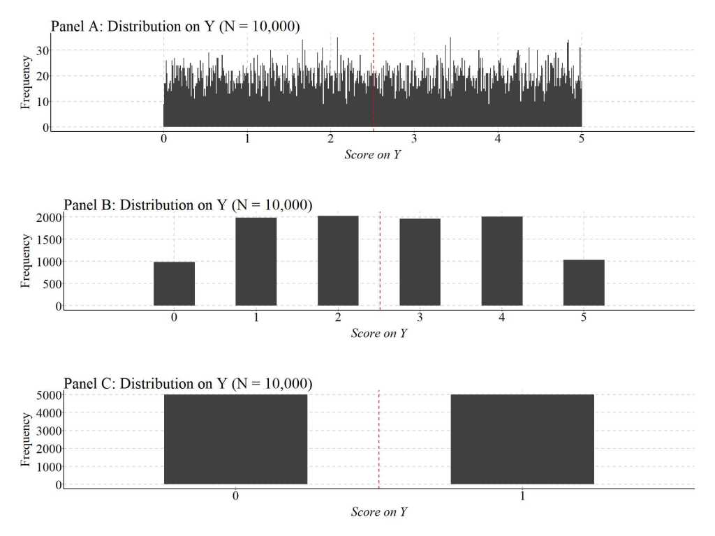
Figure 1 provides an example of the reduction in information captured in a construct as the operationalization moves from continuous to dichotomous. Briefly, Y was created as a uniform distribution ranging between 0 and 1 with up to 6 digits. This continuous operationalization of Y means that the number of expected values in the distribution is (56)10 or 8.673617e+41 value units.[iv] Panel A below was created with .01 scaled bins, meaning that we are not visually evaluating the distribution beyond 2 decimal places. That, however, does not matter as the general form of the continuous distribution is evident below. As demonstrated, it appears that only a limited number of cases fall within the 2 decimal place bins, with some bins possessing less than 10 cases and some bins possessing more than 30 cases. Moreover, we can see a substantial amount of variation in the frequency of scores on Y across the expected values of Y.
Now, let’s focus on Panel B, where scores on Y were rounded to the nearest whole number. If we treat the information about Y contained within Panel B separate from the information in Panel A, we still observe the frequency of scores on Y across the expected values of Y. Nevertheless, when compared to Panel A, the variation in the frequency of scores on Y across the expected values of Y is substantially limited,. In particular, approximately 2000 cases score 1, 2, 3, or 4 on Y (respectively) and approximately 1000 cases score 0 or 5 on Y (respectively). The reduction in the variation in the frequency of scores on Y across the expected values of Y – a loss of variation – corresponds to the reduction in information that occurs when moving from a continuous operationalization to an ordered operationalization. The reduction in the variation in the frequency of scores on Y across the expected values of Y is even further reduced in Panel C – a dichotomous operationalization of Y –, were an equal number of cases scored 0 and 1.
[Figure 1]
Now, that we understand this loss of information let us conduct various simulations to explore how altering the level of measurement and/or conducting data transformations on the dependent variable can influence the estimated effects of X on Y in our statistical models.
Brief Note: If a construct is initially operationalized at a lower level of measurement (dichotomous or ordered), you can not regain the lost variation. That is, you can not transform scores on a construct from a dichotomy to ordered to continuous or from ordered to continuous. You can only transform scores on constructs from higher levels of measurement to lower levels of measurement. Considering this, it is best to measure constructs as continuous when collecting data and then create ordered or dichotomous operationalizations if theoretically and/or empirically relevant.
2.3. Continuous Operationalization of Y
Whew, I never thought we would get here! So, let’s make this simulation as simple as possible. We are going to conduct a simple bivariate simulation, where a 1 point change in X (a normally distributed variable with a mean of 0 and standard deviation of 10) causes a 1 point change in Y (a normally distributed variable with a mean of 0 and standard deviation of 30). We place both variables in a dataframe labeled as DF. Oh, by the way, we are working with 10,000 cases.
# Continuous Construct (Linear Association) ####
n<-10000

set.seed(1992)

X<-1*rnorm(n,0,10)
Y<-1*X+1*rnorm(n,0,30)

DF<-data.frame(X,Y)
Briefly, let’s use stat.desc(DF) to ensure both constructs are continuous with the specified means and standard deviations.
> stat.desc(DF)
                                X                   Y
nbr.val      10000.00000000000000 10000.0000000000000
nbr.null         0.00000000000000     0.0000000000000
nbr.na           0.00000000000000     0.0000000000000
min            -39.07330748828923  -145.9427130332870
max             39.36370511012955   122.8730438722921
range           78.43701259841879   268.8157569055791
sum           1341.34631652977782  -724.4569705432502
median           0.00749561623815     0.0266760098151
mean             0.13413463165298    -0.0724456970543
SE.mean          0.10003327704085     0.3180169884958
CI.mean.0.95     0.19608535605966     0.6233773027025
var            100.06656515531016  1011.3480497191558
std.dev         10.00332770408478    31.8016988495765
coef.var        74.57677097115814  -438.9729154752876
As estimated below, the Spearman correlation coefficient between X and Y is equal to .31.
> corr.test(DF$X,DF$Y, method = "spearman")
Call:corr.test(x = DF$X, y = DF$Y, method = "spearman")
Correlation matrix
[1] 0.31
Sample Size
[1] 10000
These are the unadjusted probability values.
  The probability values  adjusted for multiple tests are in the p.adj object.
[1] 0

 To see confidence intervals of the correlations, print with the short=FALSE option
Now, let’s estimate our regression model and pull the key statistics. First, focusing on the specification of the regression, it can be observed that we estimated a generalized linear model (glm) while specifying that the distribution of the dependent variable is gaussian. Looking at the model results, the slope coefficient (b) for the association between X and Y was 1.054 (SE = .030), suggesting a 1 point change in X caused a 1.054 change in Y.
Briefly, the linearHypothesis function directly tests the likelihood of the slope coefficient being different from a specified value – in this case 0 – using the x2-statistics. This is extremely useful, as the x2-statistic can be used to test the similarity of coefficients across like models (e.g., a single type of model) or provide a standardized comparison of the estimated slope coefficient to a slope coefficient of 0.
The t– statistic of the estimated effects of X on Y was 35.143, while the x2– statistic of the estimated effects of X on Y was 1235.034. In this case, both tests provide evidence that the slope coefficient of the association between X and Y was statistically different from zero.
> M1<-glm(Y~X, data = DF, family = gaussian(link = "identity"))
>
> # Model Results
> summary(M1)

Call:
glm(formula = Y ~ X, family = gaussian(link = "identity"), data = DF)

Deviance Residuals:
          Min             1Q         Median             3Q            Max
-129.75743633   -20.01790880     0.07065325    20.26479953   115.13226023

Coefficients:
                Estimate   Std. Error  t value             Pr(>|t|)
(Intercept) -0.213841897  0.300067599 -0.71265              0.47608
X            1.054136418  0.029995581 35.14306 < 0.0000000000000002 ***
---
Signif. codes:  0 ‘***’ 0.001 ‘**’ 0.01 ‘*’ 0.05 ‘.’ 0.1 ‘ ’ 1

(Dispersion parameter for gaussian family taken to be 900.243756876)

    Null deviance: 10112469.149  on 9999  degrees of freedom
Residual deviance:  9000637.081  on 9998  degrees of freedom
AIC: 96409.42614

Number of Fisher Scoring iterations: 2

>
> # Chi-Square Test
> linearHypothesis(M1,c("X = 0"))
Linear hypothesis test

Hypothesis:
X = 0

Model 1: restricted model
Model 2: Y ~ X

  Res.Df Df      Chisq             Pr(>Chisq)
1   9999
2   9998  1 1235.03447 < 0.000000000000000222 ***
---
Signif. codes:  0 ‘***’ 0.001 ‘**’ 0.01 ‘*’ 0.05 ‘.’ 0.1 ‘ ’ 1
>
Now that we have the estimates corresponding to the effects of X on the continuous operationalization of Y, let’s estimate the effects of X on dichotomous and ordered operationalizations of Y.
2.4. Dichotomous Y: Version 1
For the first dichotomous operationalization of Y, we can split the distribution at the median providing a value of “1” to cases that scored above the median of Y and a value of “0” to cases that scored below or equal to the median of Y. Given that we split the distribution of Y at the median, an equal number of cases received a “0” or “1.”
> ## Dichotomous Recode 1 ####
> summary(DF$Y)
           Min.         1st Qu.          Median            Mean         3rd Qu.            Max.
-145.9427130333  -21.3951226685    0.0266760098   -0.0724456971   21.3101884312  122.8730438723
> DF$Y_DI1<-NA
> DF$Y_DI1[DF$Y<=median(DF$Y)]<-0
> DF$Y_DI1[DF$Y>median(DF$Y)]<-1
> summary(DF$Y_DI1)
   Min. 1st Qu.  Median    Mean 3rd Qu.    Max.
    0.0     0.0     0.5     0.5     1.0     1.0
> table(DF$Y_DI1)

   0    1
5000 5000
>
Now, we can estimate the Spearman correlation coefficient between X and Y_DI1 (the dichotomous operationalization of Y). The Spearman correlation coefficient is equal to .26, which is approximately .05 smaller than the Spearman correlation coefficient between X and Y.
> corr.test(DF$X,DF$Y_DI1, method = "spearman")
Call:corr.test(x = DF$X, y = DF$Y_DI1, method = "spearman")
Correlation matrix
[1] 0.26
Sample Size
[1] 10000
These are the unadjusted probability values.
  The probability values  adjusted for multiple tests are in the p.adj object.
[1] 0

 To see confidence intervals of the correlations, print with the short=FALSE option
Now, let’s estimate a binary logistic regression model and pull the key statistics. For the binary operationalization of Y, we estimated a generalized linear model (glm) while specifying that the dependent variable has a binomial distribution. Looking at the model results, the slope coefficient (b) for the association between X and Y_DI1 was 0.057 (SE = .002), suggesting a 1 point change in X caused a .057 change in Y_DI1. These estimates, however, can not be directly compared to the results of Y regressed on X because the slope coefficient will vary due to the estimator of the model.
That said, we can look at the z-statistic and x2-statistic to understand if the magnitude of the effects of X on Y_DI1 varies between the two models. The z-statistic of the estimated effects of X on Y_DI1 was 25.730, while the x2-statistic was 662.046. While the results of these tests still provide evidence that the slope coefficient of the association between X and Y_DI1 was statistically different from zero, the magnitude of the slope coefficient of X on Y_DI1 being different than zero is attenuated when compared to the magnitude of the slope coefficient of X on Y being different than zero. This suggests that recoding Y into Y_DI1 resulted in a loss of variation.
> ### Appropriate Model
> M2<-glm(Y_DI1~X,data = DF, family = binomial(link="logit"))
>
> # Model Results
> summary(M2)

Call:
glm(formula = Y_DI1 ~ X, family = binomial(link = "logit"), data = DF)

Deviance Residuals:
          Min             1Q         Median             3Q            Max
-1.9309245663  -1.1113985191  -0.0001803579   1.1130285916   1.9772226014

Coefficients:
                  Estimate     Std. Error  z value             Pr(>|z|)
(Intercept) -0.00747164118  0.02075348924 -0.36002              0.71883
X            0.05728121156  0.00222621940 25.73026 < 0.0000000000000002 ***
---
Signif. codes:  0 ‘***’ 0.001 ‘**’ 0.01 ‘*’ 0.05 ‘.’ 0.1 ‘ ’ 1

(Dispersion parameter for binomial family taken to be 1)

    Null deviance: 13862.94361  on 9999  degrees of freedom
Residual deviance: 13127.49903  on 9998  degrees of freedom
AIC: 13131.49903

Number of Fisher Scoring iterations: 4

>
> # Chi-Square Test
> linearHypothesis(M2,c("X = 0"))
Linear hypothesis test

Hypothesis:
X = 0

Model 1: restricted model
Model 2: Y_DI1 ~ X

  Res.Df Df     Chisq             Pr(>Chisq)
1   9999
2   9998  1 662.04646 < 0.000000000000000222 ***
---
Signif. codes:  0 ‘***’ 0.001 ‘**’ 0.01 ‘*’ 0.05 ‘.’ 0.1 ‘ ’ 1
2.5. Dichotomous Y: Version 2
For the second dichotomous operationalization of Y, we split the distribution at the 1st quartile of the distribution on Y. Specifically, we provided a value of “1” to cases that scored above the 1st quartile on Y and a value of “0” to cases that scored below or equal to the 1st quartile on Y. Using this recoding process, three-quarters of the cases received a value of “1” while 1-quarter of cases received a value of “0.”
> ## Dichotomous Recode 2 ####
> summary(DF$Y)
           Min.         1st Qu.          Median            Mean         3rd Qu.            Max.
-145.9427130333  -21.3951226685    0.0266760098   -0.0724456971   21.3101884312  122.8730438723
> DF$Y_DI2<-NA
> DF$Y_DI2[DF$Y<=quantile(DF$Y,.25)]<-0
> DF$Y_DI2[DF$Y>quantile(DF$Y,.25)]<-1
> summary(DF$Y_DI2)
   Min. 1st Qu.  Median    Mean 3rd Qu.    Max.
   0.00    0.75    1.00    0.75    1.00    1.00
> table(DF$Y_DI2)

   0    1
2500 7500
The Spearman correlation coefficient between X and Y_DI2 was equal to .23, which is approximately .08 smaller than the Spearman correlation coefficient between X and Y.
> corr.test(DF$X,DF$Y_DI2, method = "spearman")
Call:corr.test(x = DF$X, y = DF$Y_DI2, method = "spearman")
Correlation matrix
[1] 0.23
Sample Size
[1] 10000
These are the unadjusted probability values.
  The probability values  adjusted for multiple tests are in the p.adj object.
[1] 0

 To see confidence intervals of the correlations, print with the short=FALSE option
>
Turning to our binary logistic regression model, the slope coefficient (b) for the association between X and Y_DI2 was 0.058 (SE = .003), suggesting a 1 point change in X caused a .058 change in Y_DI2. The z-statistic of the estimated effects of X on Y_DI2 was 22.925, while the x2-statistic was 525.560. Similar to the first recode, these results suggest that recoding Y into Y_DI2 resulted in a loss of variation.
> ### Appropriate Model
> M3<-glm(Y_DI2~X,data = DF, family = binomial(link="logit"))
>
> # Model Results
> summary(M3)

Call:
glm(formula = Y_DI2 ~ X, family = binomial(link = "logit"), data = DF)

Deviance Residuals:
          Min             1Q         Median             3Q            Max
-2.4283659845  -0.0026699768   0.6343058479   0.7897773859   1.5895968726

Coefficients:
                 Estimate    Std. Error z value               Pr(>|z|)
(Intercept) 1.17040134187 0.02459766919 47.5818 < 0.000000000000000222 ***
X           0.05798629529 0.00252938007 22.9251 < 0.000000000000000222 ***
---
Signif. codes:  0 ‘***’ 0.001 ‘**’ 0.01 ‘*’ 0.05 ‘.’ 0.1 ‘ ’ 1

(Dispersion parameter for binomial family taken to be 1)

    Null deviance: 11246.70289  on 9999  degrees of freedom
Residual deviance: 10671.48756  on 9998  degrees of freedom
AIC: 10675.48756

Number of Fisher Scoring iterations: 4

> # Chi-Square Test
> linearHypothesis(M3,c("X = 0"))
Linear hypothesis test

Hypothesis:
X = 0

Model 1: restricted model
Model 2: Y_DI2 ~ X

  Res.Df Df     Chisq             Pr(>Chisq)
1   9999
2   9998  1 525.56029 < 0.000000000000000222 ***
---
Signif. codes:  0 ‘***’ 0.001 ‘**’ 0.01 ‘*’ 0.05 ‘.’ 0.1 ‘ ’ 1
>
2.6. Dichotomous Y: Version 3
For the third dichotomous operationalization of Y, we split the distribution at the score of 90. Specifically, we provided a value of “1” to cases that scored above 90 on Y and a value of “0” to cases that scored below or equal to 90 on Y. Using this recoding process, 24 cases received a value of “1” while 9,976 cases received a value of “0.”
> ## Dichotomous Recode 3 ####
> summary(DF$Y)
           Min.         1st Qu.          Median            Mean         3rd Qu.            Max.
-145.9427130333  -21.3951226685    0.0266760098   -0.0724456971   21.3101884312  122.8730438723
> DF$Y_DI3<-NA
> DF$Y_DI3[DF$Y<=90]<-0
> DF$Y_DI3[DF$Y>90]<-1
> summary(DF$Y_DI3)
   Min. 1st Qu.  Median    Mean 3rd Qu.    Max.
 0.0000  0.0000  0.0000  0.0024  0.0000  1.0000
> table(DF$Y_DI3)

   0    1
9976   24
>
We can now estimate the Spearman correlation coefficient between X and Y_DI3. The Spearman correlation coefficient is equal to .03, which is approximately .28 smaller than the Spearman correlation coefficient between X and Y.
> corr.test(DF$X,DF$Y_DI3, method = "spearman")
Call:corr.test(x = DF$X, y = DF$Y_DI3, method = "spearman")
Correlation matrix
[1] 0.03
Sample Size
[1] 10000
These are the unadjusted probability values.
  The probability values  adjusted for multiple tests are in the p.adj object.
[1] 0

 To see confidence intervals of the correlations, print with the short=FALSE option
>
Turning to our binary logistic regression model, the slope coefficient (b) for the association between X and Y_DI3 was 0.077 (SE = .021), suggesting a 1 point change in X caused a .077 change in Y_DI3. The z-statistic of the estimated effects of X on Y_DI3 was 3.765, while the x2-statistic was 14.174. These findings, again, suggest that the magnitude of the slope coefficient of X on Y_DI3 being different than zero is substantially attenuated when compared to the magnitude of the slope coefficient of X on Y being different than zero. Moreover, recoding Y into Y_DI3 resulted in a meaningful loss of variation.
> ### Appropriate Model
> M4<-glm(Y_DI3~X,data = DF, family = binomial(link="logit"))
>
> # Model Results
> summary(M4)

Call:
glm(formula = Y_DI3 ~ X, family = binomial(link = "logit"), data = DF)

Deviance Residuals:
         Min            1Q        Median            3Q           Max
-0.271194656  -0.077576747  -0.059253833  -0.045740183   3.850366527

Coefficients:
                 Estimate    Std. Error   z value               Pr(>|z|)
(Intercept) -6.3398628579  0.2605147236 -24.33591 < 0.000000000000000222 ***
X            0.0776177392  0.0206159534   3.76494             0.00016659 ***
---
Signif. codes:  0 ‘***’ 0.001 ‘**’ 0.01 ‘*’ 0.05 ‘.’ 0.1 ‘ ’ 1

(Dispersion parameter for binomial family taken to be 1)

    Null deviance: 337.4921079  on 9999  degrees of freedom
Residual deviance: 323.1462601  on 9998  degrees of freedom
AIC: 327.1462601

Number of Fisher Scoring iterations: 9

> # Chi-Square Test
> linearHypothesis(M4,c("X = 0"))
Linear hypothesis test

Hypothesis:
X = 0

Model 1: restricted model
Model 2: Y_DI3 ~ X

  Res.Df Df    Chisq Pr(>Chisq)
1   9999
2   9998  1 14.17474 0.00016659 ***
---
Signif. codes:  0 ‘***’ 0.001 ‘**’ 0.01 ‘*’ 0.05 ‘.’ 0.1 ‘ ’ 1
>
2.7. Ordered Y: Version 1
For the first ordered operationalization of Y, we split the distribution into four quartiles providing a value of “1” to cases that scored between the minimum value and the 25th percentile, a value of “2” to cases that score between the 25th percentile and the median, a value of “3” to cases that scored between the median and the 75th percentile, and a value of “4” to cases that scored between the 75th percentile and the maximum value. Using this coding scheme, an equal number of cases received a “1”, “2”, “3”, or “4.”
> ## Ordered Recode 1 ####
> summary(DF$Y)
           Min.         1st Qu.          Median            Mean         3rd Qu.            Max.
-145.9427130333  -21.3951226685    0.0266760098   -0.0724456971   21.3101884312  122.8730438723
> DF$Y_OR1<-NA
> DF$Y_OR1[DF$Y>=quantile(DF$Y,0) & DF$Y < quantile(DF$Y,.25)]<-1
> DF$Y_OR1[DF$Y>=quantile(DF$Y,.25) & DF$Y < quantile(DF$Y,.50)]<-2
> DF$Y_OR1[DF$Y>=quantile(DF$Y,.50) & DF$Y < quantile(DF$Y,.75)]<-3
> DF$Y_OR1[DF$Y>=quantile(DF$Y,.75) & DF$Y <= quantile(DF$Y,1)]<-4
> summary(DF$Y_OR1)
   Min. 1st Qu.  Median    Mean 3rd Qu.    Max.
   1.00    1.75    2.50    2.50    3.25    4.00
> table(DF$Y_OR1)

   1    2    3    4
2500 2500 2500 2500
The Spearman correlation coefficient between X and Y_OR1 was equal to .30, which is approximately .01 smaller than the Spearman correlation coefficient between X and Y.
> corr.test(DF$X, DF$Y_OR1, method = "spearman")
Call:corr.test(x = DF$X, y = DF$Y_OR1, method = "spearman")
Correlation matrix
[1] 0.3
Sample Size
[1] 10000
These are the unadjusted probability values.
  The probability values  adjusted for multiple tests are in the p.adj object.
[1] 0

 To see confidence intervals of the correlations, print with the short=FALSE option
Now, let’s estimate an ordered logistic regression model (polr from the psych package is the function to estimate this model). Looking at the model results, the slope coefficient (b) for the association between X and Y_OR1 was 0.058 (SE = .002), suggesting a 1 point change in X caused a .058 change in Y_OR1.
We can look at the t-statistic and x2-statistic to understand if the magnitude of the effects of X on Y_OR1 varies between the two models. The t-statistic of the estimated effects of X on Y_OR1 was 30.443, while the x2-statistic was 926.762. These values, again, suggest that the slope coefficient of the association between X and Y_OR1 was statistically different from zero. Nevertheless, it seems that the magnitude of the slope coefficient of X on Y_OR1 being different than zero is slightly attenuated when compared to the magnitude of the slope coefficient of X on Y, but stronger when compared to X on Y_DI1, Y_DI2, or Y_DI3. This suggests that recoding Y into Y_OR1 resulted in some loss of variation, but not to the degree of the dichotomous operationalizations of Y.
> ### Appropriate Model
> M5<-polr(as.factor(Y_OR1)~X,data = DF, Hess=TRUE) # Ordered Logistic Regression
> # Model Results
> summary(M5) # Ordered Logistic Regression
Call:
polr(formula = as.factor(Y_OR1) ~ X, data = DF, Hess = TRUE)

Coefficients:
         Value    Std. Error    t value
X 0.0578087369 0.00189893143 30.4427721

Intercepts:
    Value         Std. Error    t value
1|2  -1.169513429   0.023857898 -49.019969444
2|3   0.006946834   0.020594298   0.337318290
3|4   1.184907097   0.023948396  49.477513402

Residual Deviance: 26753.3373125
AIC: 26761.3373125
> # Chi-Square Test
> linearHypothesis(M5,c("X = 0"))
Linear hypothesis test

Hypothesis:
X = 0

Model 1: restricted model
Model 2: as.factor(Y_OR1) ~ X

  Res.Df Df     Chisq             Pr(>Chisq)
1   9997
2   9996  1 926.76237 < 0.000000000000000222 ***
---
Signif. codes:  0 ‘***’ 0.001 ‘**’ 0.01 ‘*’ 0.05 ‘.’ 0.1 ‘ ’ 1
>
2.8. Ordered Y: Version 2
For the second ordered operationalization of Y, we split the distribution into four quartiles providing a value of “1” to cases that scored between the minimum value and the 50th percentile, a value of “2” to cases that score between the 50th percentile and the 60th percentile, a value of “3” to cases that scored between the 60th percentile and the 90th percentile, and a value of “4” to cases that scored between the 90th percentile and the maximum value. Using this coding scheme, 5,000 cases received a 1, 3,000 cases received a 3, 1,000 cases received a 2, and 1,000 cases received a 4.
> ## Ordered Recode 2 ####
> summary(DF$Y)
           Min.         1st Qu.          Median            Mean         3rd Qu.            Max.
-145.9427130333  -21.3951226685    0.0266760098   -0.0724456971   21.3101884312  122.8730438723
> DF$Y_OR2<-NA
> DF$Y_OR2[DF$Y>=quantile(DF$Y,0) & DF$Y < quantile(DF$Y,.50)]<-1
> DF$Y_OR2[DF$Y>=quantile(DF$Y,.50) & DF$Y < quantile(DF$Y,.60)]<-2
> DF$Y_OR2[DF$Y>=quantile(DF$Y,.60) & DF$Y < quantile(DF$Y,.90)]<-3
> DF$Y_OR2[DF$Y>=quantile(DF$Y,.90) & DF$Y <= quantile(DF$Y,1)]<-4
> summary(DF$Y_OR2)
   Min. 1st Qu.  Median    Mean 3rd Qu.    Max.
    1.0     1.0     1.5     2.0     3.0     4.0
> table(DF$Y_OR2)

   1    2    3    4
5000 1000 3000 1000
>
The Spearman correlation coefficient between X and Y_OR2 is equal to .28, which is approximately .03 smaller than the Spearman correlation coefficient between X and Y.
> corr.test(DF$X, DF$Y_OR2, method = "spearman")
Call:corr.test(x = DF$X, y = DF$Y_OR2, method = "spearman")
Correlation matrix
[1] 0.28
Sample Size
[1] 10000
These are the unadjusted probability values.
  The probability values  adjusted for multiple tests are in the p.adj object.
[1] 0

 To see confidence intervals of the correlations, print with the short=FALSE option
>
Looking at the model results, the slope coefficient (b) for the association between X and Y_OR2 was 0.058 (SE = .002), suggesting a 1 point change in X caused a .058 change in Y_OR2. The t-statistic of the estimated effects of X on Y_OR2 was 28.697, while the x2-statistic was 823.511. These values, again, suggest that recoding Y into Y_OR2 resulted in some loss of variation, but not to the degree of the dichotomous operationalizations of Y.
> ### Appropriate Model
> M6<-polr(as.factor(Y_OR2)~X,data = DF, Hess=TRUE) # Ordered Logistic Regression
> # Model Results
> summary(M6) # Ordered Logistic Regression
Call:
polr(formula = as.factor(Y_OR2) ~ X, data = DF, Hess = TRUE)

Coefficients:
         Value   Std. Error    t value
X 0.0584219241 0.0020358283 28.6968818

Intercepts:
    Value        Std. Error   t value
1|2  0.005488792  0.020702430  0.265127913
2|3  0.441008060  0.021172836 20.828955441
3|4  2.334060459  0.034512266 67.629882084

Residual Deviance: 22484.9999904
AIC: 22492.9999904
> # Chi-Square Test
> linearHypothesis(M6,c("X = 0"))
Linear hypothesis test

Hypothesis:
X = 0

Model 1: restricted model
Model 2: as.factor(Y_OR2) ~ X

  Res.Df Df     Chisq             Pr(>Chisq)
1   9997
2   9996  1 823.51103 < 0.000000000000000222 ***
---
Signif. codes:  0 ‘***’ 0.001 ‘**’ 0.01 ‘*’ 0.05 ‘.’ 0.1 ‘ ’ 1
>
2.9. Ordered Y: Version 3
For the third ordered operationalization of Y, we split the distribution into four quartiles providing a value of “1” to cases that scored between the minimum value and the 10th percentile, a value of “2” to cases that score between the 10th percentile and the 20th percentile, a value of “3” to cases that scored between the 20th percentile and the 30th percentile, and a value of “4” to cases that scored between the 30th percentile and the maximum value. Using this coding scheme, 7,000 cases received a 4, 1,000 cases received a 1, 1,000 cases received a 2, and 1,000 cases received a 3.
> ## Ordered Recode 3 ####
> summary(DF$Y)
           Min.         1st Qu.          Median            Mean         3rd Qu.            Max.
-145.9427130333  -21.3951226685    0.0266760098   -0.0724456971   21.3101884312  122.8730438723
> DF$Y_OR3<-NA
> DF$Y_OR3[DF$Y>=quantile(DF$Y,0) & DF$Y < quantile(DF$Y,.10)]<-1
> DF$Y_OR3[DF$Y>=quantile(DF$Y,.10) & DF$Y < quantile(DF$Y,.20)]<-2
> DF$Y_OR3[DF$Y>=quantile(DF$Y,.20) & DF$Y < quantile(DF$Y,.30)]<-3
> DF$Y_OR3[DF$Y>=quantile(DF$Y,.30) & DF$Y <= quantile(DF$Y,1)]<-4
> summary(DF$Y_OR3)
   Min. 1st Qu.  Median    Mean 3rd Qu.    Max.
    1.0     3.0     4.0     3.4     4.0     4.0
> table(DF$Y_OR3)

   1    2    3    4
1000 1000 1000 7000
>
Now, we can estimate the Spearman correlation coefficient between X and Y_OR3. The Spearman correlation coefficient is equal to .25, which is approximately .06 smaller than the Spearman correlation coefficient between X and Y.
> corr.test(DF$X, DF$Y_OR3, method = "spearman")
Call:corr.test(x = DF$X, y = DF$Y_OR3, method = "spearman")
Correlation matrix
[1] 0.25
Sample Size
[1] 10000
These are the unadjusted probability values.
  The probability values  adjusted for multiple tests are in the p.adj object.
[1] 0

 To see confidence intervals of the correlations, print with the short=FALSE option
>
Looking at the model results, the slope coefficient (b) for the association between X and Y_OR3 was 0.059 (SE = .002), suggesting a 1 point change in X caused a .059 change in Y_OR3. The t-statistic of the estimated effects of X on Y_OR3 was 25.455, while the x2-statistic was 647.965. These values, again, suggest that recoding Y into Y_OR3 resulted in some loss of variation, but not to the degree of the dichotomous operationalizations of Y.
> ### Appropriate Model
> M7<-polr(as.factor(Y_OR3)~X,data = DF, Hess=TRUE) # Ordered Logistic Regression
> # Model Results
> summary(M7) # Ordered Logistic Regression
Call:
polr(formula = as.factor(Y_OR3) ~ X, data = DF, Hess = TRUE)

Coefficients:
        Value    Std. Error    t value
X 0.059398525 0.00233345826 25.4551478

Intercepts:
    Value         Std. Error    t value
1|2  -2.318094970   0.034730391 -66.745433332
2|3  -1.470420539   0.026333788 -55.837791427
3|4  -0.900170441   0.023020774 -39.102527996

Residual Deviance: 18109.1629174
AIC: 18117.1629174
> # Chi-Square Test
> linearHypothesis(M7,c("X = 0"))
Linear hypothesis test

Hypothesis:
X = 0

Model 1: restricted model
Model 2: as.factor(Y_OR3) ~ X

  Res.Df Df     Chisq             Pr(>Chisq)
1   9997
2   9996  1 647.96455 < 0.000000000000000222 ***
---
Signif. codes:  0 ‘***’ 0.001 ‘**’ 0.01 ‘*’ 0.05 ‘.’ 0.1 ‘ ’ 1
>
2.10. Summary of Results
As introduced above, recoding a construct from a continuous distribution to an ordered distribution or a binomial distribution results in the reduction in the variation in the frequency of scores on Y across the expected values of Y. This is evident in the simulated results, as the t-statistics, z-statistics, and x2-statistics appear to be attenuated when moving from a continuous operationalization of the dependent variable to an ordered or dichotomous operationalization. When implementing a statistical model with appropriate assumptions about the distribution of scores on the dependent variable, this loss of variation has limited impact on the slope coefficient but could result in an increased likelihood of committing a Type 1 or Type 2 error. Specifically, moving across levels of measurement for the dependent variable directly impacts our ability to conduct an accurate hypothesis test. While the simulated demonstrations presented above did not result in a Type 1 or Type 2 error, a variety of recoding processes can result in the hypothesis test suggesting an association opposite of the causal association in the population. This is most concerning when a causal association between two continuous constructs does not exist within the population, but regressing a non-continuous operationalization of the dependent variable on the independent variable produces a hypothesis test suggesting an association exists within the population (i.e., a Type 1 error). Overall, the results of the first set of simulations suggest that we should be cautious when and/or actively try not to recode our dependent variable from a continuous operationalization to an ordered or dichotomous operationalization unless theoretical or empirical justification exists.
3. Data Transformations
Now that we have completed our discussion about altering the level of measurement of the dependent variable, let’s discuss data transformations. Okay, so in my opinion, a data transformation refers to the process of recoding a construct to alter the structure or scale of the distribution, while maintaining a continuous operationalization of the construct. That is, a data transformation is a subtype of recoding process used when cleaning data. Unlike the recodes performed in the previous section, all data transformations will maintain variation in the frequency of scores on Y across the expected values of Y. Nevertheless, data transformations alter the distribution of scores by either changing the scale or structure of the distribution. As such, these techniques are commonly used to satisfy the assumptions of statistical models.
While the largest concern with most data transformations is the inability to interpret the slope coefficient on the raw scale of the dependent variable, some data transformations can change the rank order of a distribution. That is, for example, a case with the lowest score on a test could become ranked higher than the lowest score after the implementation of certain data transformations. Altering the rank order of a distribution could generate the inability to observe the causal association between X and Y within the population. A similar problem arises when we restrict the distribution of scores to minimum and maximum values not representative of the distribution in the population. That is, if we exclude the case with the lowest score on a test from an analysis solely because we restrict the possible scores that we want to examine. Conducting this data transformation, similarly, can generate the inability to observe the causal association between X and Y within the population.
As a reminder, the Spearman correlation coefficient between X and Y was .31, the slope coefficient (b) for the association between X and Y was 1.054 (SE = .030), the t-statistic of the estimated effects of X on Y was 35.143, and the x2-statistic of the estimated effects of X on Y was 1235.034.
3.1. Multiplying by A Constant
To be honest, this is the data transformation I frequently use when estimating a structural equation model (SEM). This technique is most beneficial when the data being analyzed possesses an ill-scaled covariance matrix (i.e., some variances/covariances are substantially larger or smaller than other variances/covariances). We can go into more detail about how this works when discussing multilevel modeling or SEM but, briefly, scaling the covariance matrix properly increases the probability of a multilevel model or SEM model converging upon a single solution.
Multiplying a continuous distribution by any constant simply shifts the distribution up or down the x-axis. When the constant is a decimal smaller than one the distribution will shift down the x-axis and the variance will become smaller. When the constant is a number larger than one the distribution will shift up the x-axis and the variance will become larger. Generally, in my research, I stick to constants that start with a 1 and are all zeros (e.g., 10, 100, 1000), constants that are all zeros and end in 1 (e.g., .01, .001, .0001), or .1 to maintain the interpretability of the slope coefficient within the scale of the original measure. Either way, while the slope coefficient (b) and standard error (SE) will change, the correlation coefficient, the standardized effects of X on Y (β), the t– statistic, and the x2– statistic will remain constant using this type of transformation.
3.1.1. Example 1: Y*.2
In this first example, we multiply Y by .2 to create Y_Re.2. Evident by the results, the Spearman correlation coefficient between X and Y_Re.2 was .31, the slope coefficient (b) was .211 (SE = .006), the t– statistic was 35.143, and the x2– statistic was 1235.034. As expected, the Spearman correlation coefficient, the t– statistic, and the x2– statistic are identical to the values observed when estimating the association between X and Y.
> ### Example 1: Rescaled by .2
> DF$Y_Re.2<-Y*.2
> summary(DF$Y_Re.2)
           Min.         1st Qu.          Median            Mean         3rd Qu.            Max.
-29.18854260666  -4.27902453369   0.00533520196  -0.01448913941   4.26203768624  24.57460877446
>
>
> corr.test(DF$X,DF$Y_Re.2, method = "spearman")
Call:corr.test(x = DF$X, y = DF$Y_Re.2, method = "spearman")
Correlation matrix
[1] 0.31
Sample Size
[1] 10000
These are the unadjusted probability values.
  The probability values  adjusted for multiple tests are in the p.adj object.
[1] 0

 To see confidence intervals of the correlations, print with the short=FALSE option
>
> M2<-glm(Y_Re.2~X, data = DF, family = gaussian(link = "identity"))
>
> # Model Results
> summary(M2)

Call:
glm(formula = Y_Re.2 ~ X, family = gaussian(link = "identity"),
    data = DF)

Deviance Residuals:
          Min             1Q         Median             3Q            Max
-25.951487265   -4.003581759    0.014130651    4.052959907   23.026452047

Coefficients:
                 Estimate    Std. Error  t value             Pr(>|t|)
(Intercept) -0.0427683794  0.0600135198 -0.71265              0.47608
X            0.2108272836  0.0059991162 35.14306 < 0.0000000000000002 ***
---
Signif. codes:  0 ‘***’ 0.001 ‘**’ 0.01 ‘*’ 0.05 ‘.’ 0.1 ‘ ’ 1

(Dispersion parameter for gaussian family taken to be 36.009750275)

    Null deviance: 404498.7660  on 9999  degrees of freedom
Residual deviance: 360025.4832  on 9998  degrees of freedom
AIC: 64220.66789

Number of Fisher Scoring iterations: 2

> # Chi-Square Test
> linearHypothesis(M2,c("X = 0"))
Linear hypothesis test

Hypothesis:
X = 0

Model 1: restricted model
Model 2: Y_Re.2 ~ X

  Res.Df Df      Chisq             Pr(>Chisq)
1   9999
2   9998  1 1235.03447 < 0.000000000000000222 ***
---
Signif. codes:  0 ‘***’ 0.001 ‘**’ 0.01 ‘*’ 0.05 ‘.’ 0.1 ‘ ’ 1
>
3.1.2. Example 1: Y*20
In this second example, we multiply Y by 20 to create Y_Re2. Evident by the results, the Spearman correlation coefficient between X and Y_Re2 was .31, the slope coefficient (b) was 21.083 (SE = .600), the t– statistic was 35.143, and the x2– statistic was 1235.034. Similar to the previous example, the Spearman correlation coefficient, the t– statistic, and the x2– statistic are identical to the values observed when estimating the association between X and Y.
> ### Example 2: Rescaled by 20
> DF$Y_Re2<-Y*20
> summary(DF$Y_Re2)
           Min.         1st Qu.          Median            Mean         3rd Qu.            Max.
-2918.854260666  -427.902453369     0.533520196    -1.448913941   426.203768624  2457.460877446
>
>
> corr.test(DF$X,DF$Y_Re2, method = "spearman")
Call:corr.test(x = DF$X, y = DF$Y_Re2, method = "spearman")
Correlation matrix
[1] 0.31
Sample Size
[1] 10000
These are the unadjusted probability values.
  The probability values  adjusted for multiple tests are in the p.adj object.
[1] 0

 To see confidence intervals of the correlations, print with the short=FALSE option
>
> M3<-glm(Y_Re2~X, data = DF, family = gaussian(link = "identity"))
>
> # Model Results
> summary(M3)

Call:
glm(formula = Y_Re2 ~ X, family = gaussian(link = "identity"),
    data = DF)

Deviance Residuals:
          Min             1Q         Median             3Q            Max
-2595.1487265   -400.3581759      1.4130651    405.2959907   2302.6452047

Coefficients:
               Estimate  Std. Error  t value             Pr(>|t|)
(Intercept) -4.27683794  6.00135198 -0.71265              0.47608
X           21.08272836  0.59991162 35.14306 < 0.0000000000000002 ***
---
Signif. codes:  0 ‘***’ 0.001 ‘**’ 0.01 ‘*’ 0.05 ‘.’ 0.1 ‘ ’ 1

(Dispersion parameter for gaussian family taken to be 360097.50275)

    Null deviance: 4044987660  on 9999  degrees of freedom
Residual deviance: 3600254832  on 9998  degrees of freedom
AIC: 156324.0716

Number of Fisher Scoring iterations: 2

> # Chi-Square Test
> linearHypothesis(M3,c("X = 0"))
Linear hypothesis test

Hypothesis:
X = 0

Model 1: restricted model
Model 2: Y_Re2 ~ X

  Res.Df Df      Chisq             Pr(>Chisq)
1   9999
2   9998  1 1235.03447 < 0.000000000000000222 ***
---
Signif. codes:  0 ‘***’ 0.001 ‘**’ 0.01 ‘*’ 0.05 ‘.’ 0.1 ‘ ’ 1
>
3.2. Standardizing Scores on Y
Okay, so this example is a little unnecessary because the distribution of Y is already normal, but a common continuous data transformation is z-scoring the distribution for the dependent variable – “z-scoring” sounds weird, but we will roll with it! This transformation generates a continuous normal distribution from the variable being transformed, were a 1 unit change in the variable now corresponds to a 1 standard deviation change in the variable. R makes it easy to conduct this data transformation with the scale() function.
Given that Y is already normal, the slope coefficient (b) and standard error (SE) will change, but the correlation coefficient, the standardized effects of X on Y (β), the t– statistic, and the x2– statistic will remain constant. That said, if you z-score a non-normal distribution it is possible for all of the coefficients, including the correlation coefficient, the standardized effects of X on Y (β), the t– statistic, and the x2– statistic, to change. Z-scores are invasive data transformations when working with non-normal distributions as they alter the shape or rank order of the distribution.
In this example, we z-scored Y using the scale() function and created Y_z. Evident by the results, the Spearman correlation coefficient between X and Y_z was .31, the slope coefficient (b) for the association between X and Y_z was .033 (SE = .001), the t– statistic was 35.143, and the x2– statistic was 1235.034. As expected, the Spearman correlation coefficient, the t– statistic, and the x2– statistic are identical to the values observed when estimating the association between X and Y. When using this transformation, the slope coefficient is interpreted as a 1 unit change in X results in a .033 standard deviation change in Y.
> ## Standardizing Data ####
> DF$Y_z<-scale(DF$Y)
> summary(DF$Y_z)
       V1
 Min.   :-4.58687028093
 1st Qu.:-0.67048861359
 Median : 0.00311686829
 Mean   : 0.00000000000
 3rd Qu.: 0.67237395805
 Max.   : 3.86600383051
>
> corr.test(DF$X,DF$Y_z, method = "spearman")
Call:corr.test(x = DF$X, y = DF$Y_z, method = "spearman")
Correlation matrix
     [,1]
[1,] 0.31
Sample Size
[1] 10000
These are the unadjusted probability values.
  The probability values  adjusted for multiple tests are in the p.adj object.
     [,1]
[1,]    0

 To see confidence intervals of the correlations, print with the short=FALSE option
>
> M4<-glm(Y_z~X, data = DF, family = gaussian(link = "identity"))
>
> # Model Results
> summary(M4)

Call:
glm(formula = Y_z ~ X, family = gaussian(link = "identity"),
    data = DF)

Deviance Residuals:
         Min            1Q        Median            3Q           Max
-4.080204549  -0.629460360   0.002221682   0.637223805   3.620317920

Coefficients:
                   Estimate      Std. Error  t value            Pr(>|t|)
(Intercept) -0.004446183860  0.009435583934 -0.47121              0.6375
X            0.033147173144  0.000943206876 35.14306 <0.0000000000000002 ***
---
Signif. codes:  0 ‘***’ 0.001 ‘**’ 0.01 ‘*’ 0.05 ‘.’ 0.1 ‘ ’ 1

(Dispersion parameter for gaussian family taken to be 0.890142376925)

    Null deviance: 9999.000000  on 9999  degrees of freedom
Residual deviance: 8899.643484  on 9998  degrees of freedom
AIC: 27219.03191

Number of Fisher Scoring iterations: 2

> # Chi-Square Test
> linearHypothesis(M4,c("X = 0"))
Linear hypothesis test

Hypothesis:
X = 0

Model 1: restricted model
Model 2: Y_z ~ X

  Res.Df Df      Chisq             Pr(>Chisq)
1   9999
2   9998  1 1235.03447 < 0.000000000000000222 ***
---
Signif. codes:  0 ‘***’ 0.001 ‘**’ 0.01 ‘*’ 0.05 ‘.’ 0.1 ‘ ’ 1
>
3.3. Normalizing Scores on Y
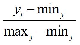
Normalizing a distribution means that we are going to take the structure of the distribution – as is – but require the scores to range between zero and one. To normalize a variable, we take each case’s score on the variable and subtract the minimum value of the distribution and divide by the difference between the maximum and minimum values of the distribution (Equation 1).
[Equation 1]
There aren’t a large number of cases where one would only normalize the distribution of a variable, as multiplying by a constant is easier when rescaling a distribution. That said, however, it is extremely important to normalize a distribution when implementing certain data transformations.
In this example, we normalized Y using equation 1 and created Y_n. Evident by the results, the Spearman correlation coefficient between X and Y_n was .31, the slope coefficient (b) for the association between X and Y_n was .004 (SE = .0001), the t– statistic was 35.143, and the x2– statistic was 1235.034. As expected, the Spearman correlation coefficient, the t– statistic, and the x2– statistic are identical to the values observed when estimating the association between X and Y.
> ## Normalizing Data ####
>
> DF$Y_n<-((DF$Y)-min(DF$Y))/((max(DF$Y))-min(DF$Y))
> summary(DF$Y_n)
       Min.     1st Qu.      Median        Mean     3rd Qu.        Max.
0.000000000 0.463319531 0.543009051 0.542640316 0.622184143 1.000000000
>
>
> corr.test(DF$X,DF$Y_n, method = "spearman")
Call:corr.test(x = DF$X, y = DF$Y_n, method = "spearman")
Correlation matrix
[1] 0.31
Sample Size
[1] 10000
These are the unadjusted probability values.
  The probability values  adjusted for multiple tests are in the p.adj object.
[1] 0

 To see confidence intervals of the correlations, print with the short=FALSE option
>
> M5<-glm(Y_n~X, data = DF, family = gaussian(link = "identity"))
>
> # Model Results
> summary(M5)

Call:
glm(formula = Y_n ~ X, family = gaussian(link = "identity"),
    data = DF)

Deviance Residuals:
          Min             1Q         Median             3Q            Max
-0.4827002621  -0.0744670217   0.0002628315   0.0753854602   0.4282943141

Coefficients:
                  Estimate     Std. Error   t value               Pr(>|t|)
(Intercept) 0.542114319538 0.001116257478 485.65347 < 0.000000000000000222 ***
X           0.003921408589 0.000111584162  35.14306 < 0.000000000000000222 ***
---
Signif. codes:  0 ‘***’ 0.001 ‘**’ 0.01 ‘*’ 0.05 ‘.’ 0.1 ‘ ’ 1

(Dispersion parameter for gaussian family taken to be 0.012458067361)

    Null deviance: 139.9419001  on 9999  degrees of freedom
Residual deviance: 124.5557575  on 9998  degrees of freedom
AIC: -15471.09839

Number of Fisher Scoring iterations: 2

> # Chi-Square Test
> linearHypothesis(M5,c("X = 0"))
Linear hypothesis test

Hypothesis:
X = 0

Model 1: restricted model
Model 2: Y_n ~ X

  Res.Df Df      Chisq             Pr(>Chisq)
1   9999
2   9998  1 1235.03447 < 0.000000000000000222 ***
---
Signif. codes:  0 ‘***’ 0.001 ‘**’ 0.01 ‘*’ 0.05 ‘.’ 0.1 ‘ ’ 1
>
3.4. Log Transformations of Y
Logarithmic data transformations are pretty invasive and require strong justification to implement. In the current context, invasive refers to data transformations that can alter the shape or rank order of a distribution. They tend to be most commonly implemented when trying to satisfy the normality assumption with a variable that is known to be positively skewed within the population. Specifically, calculating the logarithm of a variable reduces the skew within the distribution because the difference between the raw score and logarithm of the raw score become larger when the raw score is larger. To provide an example, the natural log of 10 is 2.303 and the natural log of 100,000,000 is 18.421.
This subset of data transformations is most commonly implemented when working with income. Specifically, income has an extreme positive skew within the population and can not satisfy the normality assumption. As such, we might take the log of the observed distribution to hopefully satisfy the normality assumption. Personally, I have not seen many people calculate the log of a distribution besides income, so if you have other examples please share them! That said, logarithmic data transformations are extremely finicky and might not achieve the desired goal. Moreover, as a reminder, you can not calculate the log of 0 or of negative values.
3.4.1. Base Log
In this example, we want to calculate the base log of Y. Y, however, is a normal distribution with positive and negative values. As such, there are two ways we can make the Y distribution appropriate for the base log transformation. We can 1) add a positive constant greater than the largest negative value to Y or 2) normalize the distribution on T. Given that Y_n already existed in the dataframe, we can calculate the base log of the normalized Y distribution using log(Y_n) creating Y_log. Evident by the results, the spearman correlation between X and Y_log was .31, the slope coefficient (b) was .006 (SE = .0001), the t– statistic was 34.701, and the x2– statistic was 1204.149. While the amount of variance in the distribution was slightly reduced by calculating the log of the normalized Y distribution, the reduction in variance was nominal and the results remained largely the same. Importantly, when interpreting the slope coefficient between X and Y_log, a 1 point change in X resulted in a .006 base log change in the normalized distribution of Y.
> ### Base Log
> DF$Y_n<-((DF$Y)-min(DF$Y-25))/((max(DF$Y+25))-min(DF$Y-25))
>
> DF$Y_log<-log(DF$Y_n)
> summary(DF$Y_log)
         Min.       1st Qu.        Median          Mean       3rd Qu.          Max.
-2.5457375465 -0.7569986990 -0.6231288423 -0.6422487284 -0.5058016710 -0.0816604777
>
>
> corr.test(DF$X,DF$Y_log, method = "spearman")
Call:corr.test(x = DF$X, y = DF$Y_log, method = "spearman")
Correlation matrix
[1] 0.31
Sample Size
[1] 10000
These are the unadjusted probability values.
  The probability values  adjusted for multiple tests are in the p.adj object.
[1] 0

 To see confidence intervals of the correlations, print with the short=FALSE option
>
> M6<-glm(Y_log~X, data = DF, family = gaussian(link = "identity"))
>
> # Model Results
> summary(M6)

Call:
glm(formula = Y_log ~ X, family = gaussian(link = "identity"),
    data = DF)

Deviance Residuals:
          Min             1Q         Median             3Q            Max
-1.7234362625  -0.1091117847   0.0169627735   0.1287641726   0.5672971592

Coefficients:
                   Estimate      Std. Error    t value               Pr(>|t|)
(Intercept) -0.643116285983  0.001864571499 -344.91372 < 0.000000000000000222 ***
X            0.006467811822  0.000186387686   34.70085 < 0.000000000000000222 ***
---
Signif. codes:  0 ‘***’ 0.001 ‘**’ 0.01 ‘*’ 0.05 ‘.’ 0.1 ‘ ’ 1

(Dispersion parameter for gaussian family taken to be 0.0347600182253)

    Null deviance: 389.3869119  on 9999  degrees of freedom
Residual deviance: 347.5306622  on 9998  degrees of freedom
AIC: -5210.104079

Number of Fisher Scoring iterations: 2

> # Chi-Square Test
> linearHypothesis(M6,c("X = 0"))
Linear hypothesis test

Hypothesis:
X = 0

Model 1: restricted model
Model 2: Y_log ~ X

  Res.Df Df      Chisq             Pr(>Chisq)
1   9999
2   9998  1 1204.14924 < 0.000000000000000222 ***
---
Signif. codes:  0 ‘***’ 0.001 ‘**’ 0.01 ‘*’ 0.05 ‘.’ 0.1 ‘ ’ 1
>
3.4.2. Log 10
We can calculate the log10 of the normalized Y distribution using log10(Y_n) creating Y_log10. Evident by the results, the Spearman correlation coefficient between X and Y_log10 was .31, the slope coefficient (b) was .006 (SE = .0001), the t– statistic was 34.701, and the x2– statistic was 1204.149. Again, the reduction in variance in the Y distribution was nominal and the Spearman correlation coefficient, the t– statistic, and the x2– statistic were almost identical to the values observed when estimating the association between X and Y.
> ###  Log10
> DF$Y_n<-((DF$Y)-min(DF$Y-25))/((max(DF$Y+25))-min(DF$Y-25))
>
> DF$Y_log10<-log10(DF$Y_n)
> summary(DF$Y_log10)
         Min.       1st Qu.        Median          Mean       3rd Qu.          Max.
-1.1055997688 -0.3287603578 -0.2706214177 -0.2789250788 -0.2196668747 -0.0354646948
>
> corr.test(DF$X,DF$Y_log10, method = "spearman")
Call:corr.test(x = DF$X, y = DF$Y_log10, method = "spearman")
Correlation matrix
[1] 0.31
Sample Size
[1] 10000
These are the unadjusted probability values.
  The probability values  adjusted for multiple tests are in the p.adj object.
[1] 0

 To see confidence intervals of the correlations, print with the short=FALSE option
>
> M7<-glm(Y_log10~X, data = DF, family = gaussian(link = "identity"))
>
> # Model Results
> summary(M7)

Call:
glm(formula = Y_log10 ~ X, family = gaussian(link = "identity"),
    data = DF)

Deviance Residuals:
          Min             1Q         Median             3Q            Max
-0.7484788587  -0.0473866460   0.0073668389   0.0559215696   0.2463740259

Coefficients:
                    Estimate       Std. Error    t value               Pr(>|t|)
(Intercept) -0.2793018542246  0.0008097731131 -344.91372 < 0.000000000000000222 ***
X            0.0028089349844  0.0000809471436   34.70085 < 0.000000000000000222 ***
---
Signif. codes:  0 ‘***’ 0.001 ‘**’ 0.01 ‘*’ 0.05 ‘.’ 0.1 ‘ ’ 1

(Dispersion parameter for gaussian family taken to be 0.00655614602563)

    Null deviance: 73.44292624  on 9999  degrees of freedom
Residual deviance: 65.54834796  on 9998  degrees of freedom
AIC: -21890.75298

Number of Fisher Scoring iterations: 2

> # Chi-Square Test
> linearHypothesis(M7,c("X = 0"))
Linear hypothesis test

Hypothesis:
X = 0

Model 1: restricted model
Model 2: Y_log10 ~ X

  Res.Df Df      Chisq             Pr(>Chisq)
1   9999
2   9998  1 1204.14924 < 0.000000000000000222 ***
---
Signif. codes:  0 ‘***’ 0.001 ‘**’ 0.01 ‘*’ 0.05 ‘.’ 0.1 ‘ ’ 1
>
3.5. Power Transformations—Raw Scale
Power transformations refers to the subset of data transformations calculated by raising the scores on a distribution to the nth power. Power transformations, similar to logarithm transformations, are generally invasive and could result in some unintended consequences. An example of a power transformation is Y2, where Y is raised to the second power or (Y*Y). At the forefront of issues associated with power transformations, is the potential alteration of the rank order of the distribution on Y when calculating Y2. The rank order is most commonly affected when negative values exist within the Y distribution and the variable is raised to an even power (e.g., 2, 4, 6, 8). Remember, a negative number raised to an even power equals a positive value! This is demonstrated in the simulations below, were we subject the raw scale of Y to power transformations.
3.5.1. Y Squared
In this example, we calculated Y^2 in R to create Y2. Evident by the results, the Spearman correlation coefficient between X and Y2 was 0, the slope coefficient (b) was -1.722 (SE = 1.477), the t– statistic was -1.166, and the x2– statistic was 1.359. These results are a large departure from reality and suggest that X does not have any statistical association with Y2. These results occurred because we altered the rank order in Y. For instance, the minimum value for Y – the largest negative value –has the maximum value on the distribution of Y2.
> ### Squared
> DF$Y2<-DF$Y^2
> summary(DF$Y2)
          Min.        1st Qu.         Median           Mean        3rd Qu.           Max.
    0.00002969   104.06660167   456.43430867  1011.25216329  1308.79640623 21299.27548752
>
> corr.test(DF$X,DF$Y2, method = "spearman")
Call:corr.test(x = DF$X, y = DF$Y2, method = "spearman")
Correlation matrix
[1] 0
Sample Size
[1] 10000
These are the unadjusted probability values.
  The probability values  adjusted for multiple tests are in the p.adj object.
[1] 0.91

 To see confidence intervals of the correlations, print with the short=FALSE option
>
> M8<-glm(Y2~X, data = DF, family = gaussian(link = "identity"))
>
> # Model Results
> summary(M8)

Call:
glm(formula = Y2 ~ X, family = gaussian(link = "identity"), data = DF)

Deviance Residuals:
         Min            1Q        Median            3Q           Max
-1063.781905   -908.209722   -555.471354    301.302216  20240.074412

Coefficients:
                 Estimate    Std. Error  t value             Pr(>|t|)
(Intercept) 1011.48319829   14.77947982 68.43835 < 0.0000000000000002 ***
X             -1.72241123    1.47739738 -1.16584              0.24371
---
Signif. codes:  0 ‘***’ 0.001 ‘**’ 0.01 ‘*’ 0.05 ‘.’ 0.1 ‘ ’ 1

(Dispersion parameter for gaussian family taken to be 2183937.5233)

    Null deviance: 21837975736  on 9999  degrees of freedom
Residual deviance: 21835007358  on 9998  degrees of freedom
AIC: 174349.1706

Number of Fisher Scoring iterations: 2

> # Chi-Square Test
> linearHypothesis(M8,c("X = 0"))
Linear hypothesis test

Hypothesis:
X = 0

Model 1: restricted model
Model 2: Y2 ~ X

  Res.Df Df   Chisq Pr(>Chisq)
1   9999
2   9998  1 1.35919    0.24368
>
3.5.2. Y Raised to the .2 Power
A similar result is observed when we calculate Y^.2 in R to create Y.2. The source of the problem in this condition is that we can not raise negative values to decimal powers (e.g., -2^.2). Instead, R provides an NA for these cases. This has important implications, as the Spearman correlation coefficient between X and Y.2 was .19, the slope coefficient (b) was -.006 (SE = .0005), the t– statistic was 12.827, and the x2– statistic was 164.531. These results, while better than the previous transformation, are a large departure from reality.
> ### raised to the .2 power
> DF$Y.2<-DF$Y^.2
> summary(DF$Y.2)
      Min.    1st Qu.     Median       Mean    3rd Qu.       Max.       NA's
0.35258635 1.59715625 1.84374283 1.79812642 2.04865388 2.61752792       4997
>
> corr.test(DF$X,DF$Y.2, method = "spearman")
Call:corr.test(x = DF$X, y = DF$Y.2, method = "spearman")
Correlation matrix
[1] 0.19
Sample Size
[1] 5003
These are the unadjusted probability values.
  The probability values  adjusted for multiple tests are in the p.adj object.
[1] 0

 To see confidence intervals of the correlations, print with the short=FALSE option
>
> M9<-glm(Y.2~X, data = DF, family = gaussian(link = "identity"))
>
> # Model Results
> summary(M9)

Call:
glm(formula = Y.2 ~ X, family = gaussian(link = "identity"),
    data = DF)

Deviance Residuals:
          Min             1Q         Median             3Q            Max
-1.4992221645  -0.1967287252   0.0469582285   0.2482599743   0.8157676896

Coefficients:
                  Estimate     Std. Error   t value               Pr(>|t|)
(Intercept) 1.780398448541 0.005010141910 355.35889 < 0.000000000000000222 ***
X           0.006343692745 0.000494558503  12.82698 < 0.000000000000000222 ***
---
Signif. codes:  0 ‘***’ 0.001 ‘**’ 0.01 ‘*’ 0.05 ‘.’ 0.1 ‘ ’ 1

(Dispersion parameter for gaussian family taken to be 0.116026399605)

    Null deviance: 599.3380165  on 5002  degrees of freedom
Residual deviance: 580.2480244  on 5001  degrees of freedom
  (4997 observations deleted due to missingness)
AIC: 3425.749096

Number of Fisher Scoring iterations: 2

> # Chi-Square Test
> linearHypothesis(M9,c("X = 0"))
Linear hypothesis test

Hypothesis:
X = 0

Model 1: restricted model
Model 2: Y.2 ~ X

  Res.Df Df     Chisq             Pr(>Chisq)
1   5002
2   5001  1 164.53145 < 0.000000000000000222 ***
---
Signif. codes:  0 ‘***’ 0.001 ‘**’ 0.01 ‘*’ 0.05 ‘.’ 0.1 ‘ ’ 1
>
3.6. Power Transformations—Normalized Scale
To demonstrate the results when the scale is normalized, we replicated the power transformations performed above on Y_n.
3.6.1. Y Squared
In this example, we raised Y_n^2 and created Y2_n. Evident by the results, the Spearman correlation coefficient between X and Y2_n was .31, the slope coefficient (b) was .004 (SE = .0001), the t– statistic was 34.750, and the x2– statistic was 1207.574.
> ### Squared
> DF$Y_n<-((DF$Y)-min(DF$Y-25))/((max(DF$Y+25))-min(DF$Y-25))
> DF$Y2_n<-DF$Y_n^2
> summary(DF$Y2_n)
         Min.       1st Qu.        Median          Mean       3rd Qu.          Max.
0.00614894293 0.22002867549 0.28757899690 0.29719459761 0.36363547996 0.84931855134
>
> corr.test(DF$X,DF$Y2_n, method = "spearman")
Call:corr.test(x = DF$X, y = DF$Y2_n, method = "spearman")
Correlation matrix
[1] 0.31
Sample Size
[1] 10000
These are the unadjusted probability values.
  The probability values  adjusted for multiple tests are in the p.adj object.
[1] 0

 To see confidence intervals of the correlations, print with the short=FALSE option
>
> M10<-glm(Y2_n~X, data = DF, family = gaussian(link = "identity"))
>
> # Model Results
> summary(M10)

Call:
glm(formula = Y2_n ~ X, family = gaussian(link = "identity"),
    data = DF)

Deviance Residuals:
          Min             1Q         Median             3Q            Max
-0.3214133267  -0.0721628155  -0.0082762638   0.0627939165   0.5195618085

Coefficients:
                  Estimate     Std. Error   t value               Pr(>|t|)
(Intercept) 0.296721273971 0.001015832865 292.09655 < 0.000000000000000222 ***
X           0.003528720613 0.000101545442  34.75016 < 0.000000000000000222 ***
---
Signif. codes:  0 ‘***’ 0.001 ‘**’ 0.01 ‘*’ 0.05 ‘.’ 0.1 ‘ ’ 1

(Dispersion parameter for gaussian family taken to be 0.0103173088415)

    Null deviance: 115.6113655  on 9999  degrees of freedom
Residual deviance: 103.1524538  on 9998  degrees of freedom
AIC: -17356.55278

Number of Fisher Scoring iterations: 2

> # Chi-Square Test
> linearHypothesis(M10,c("X = 0"))
Linear hypothesis test

Hypothesis:
X = 0

Model 1: restricted model
Model 2: Y2_n ~ X

  Res.Df Df      Chisq             Pr(>Chisq)
1   9999
2   9998  1 1207.57379 < 0.000000000000000222 ***
---
Signif. codes:  0 ‘***’ 0.001 ‘**’ 0.01 ‘*’ 0.05 ‘.’ 0.1 ‘ ’ 1
>
3.6.2. Y Raised to the .2 Power
In this example, we raised Y_n^.2 and created Y.2_n. Evident by the results, the Spearman correlation coefficient between X and Y.2_n was .31, the slope coefficient (b) was .001 (SE = .000), the t– statistic was 34.881, and the x2– statistic was 1216.697.
> ### raised to the .2 power
> DF$Y.2_n<-DF$Y_n^.2
> summary(DF$Y.2_n)
       Min.     1st Qu.      Median        Mean     3rd Qu.        Max.
0.601007714 0.859504052 0.882827223 0.880135741 0.903788113 0.983800550
>
> corr.test(DF$X,DF$Y.2_n, method = "spearman")
Call:corr.test(x = DF$X, y = DF$Y.2_n, method = "spearman")
Correlation matrix
[1] 0.31
Sample Size
[1] 10000
These are the unadjusted probability values.
  The probability values  adjusted for multiple tests are in the p.adj object.
[1] 0

 To see confidence intervals of the correlations, print with the short=FALSE option
>
> M11<-glm(Y.2_n~X, data = DF, family = gaussian(link = "identity"))
>
> # Model Results
> summary(M11)

Call:
glm(formula = Y.2_n ~ X, family = gaussian(link = "identity"),
    data = DF)

Deviance Residuals:
           Min              1Q          Median              3Q             Max
-0.24776294359  -0.01952569669   0.00239017516   0.02227604032   0.10308605172

Coefficients:
                   Estimate      Std. Error    t value               Pr(>|t|)
(Intercept) 0.8799846131849 0.0003231284086 2723.32791 < 0.000000000000000222 ***
X           0.0011266902551 0.0000323008029   34.88118 < 0.000000000000000222 ***
---
Signif. codes:  0 ‘***’ 0.001 ‘**’ 0.01 ‘*’ 0.05 ‘.’ 0.1 ‘ ’ 1

(Dispersion parameter for gaussian family taken to be 0.00104393196527)

    Null deviance: 11.70738069  on 9999  degrees of freedom
Residual deviance: 10.43723179  on 9998  degrees of freedom
AIC: -40264.83913

Number of Fisher Scoring iterations: 2

> # Chi-Square Test
> linearHypothesis(M11,c("X = 0"))
Linear hypothesis test

Hypothesis:
X = 0

Model 1: restricted model
Model 2: Y.2_n ~ X

  Res.Df Df      Chisq             Pr(>Chisq)
1   9999
2   9998  1 1216.69701 < 0.000000000000000222 ***
---
Signif. codes:  0 ‘***’ 0.001 ‘**’ 0.01 ‘*’ 0.05 ‘.’ 0.1 ‘ ’ 1
>
3.7. Rounding Raw Scores
Just for fun, let’s see what happens if we round the scores on Y to the nearest whole digit! In this example, we used round(Y) and created Y_R. Evident by the results, the Spearman correlation coefficient between X and Y_R was .31, the slope coefficient (b) was 1.054 (SE = .030), the t– statistic was 35.145, and the x2– statistic was 1235.153. These results are identical to the results of Y regressed on X, because simply rounding Y to the nearest whole number did not reduce the variance of the distribution. That is, the distribution of Y is continuous enough to maintain its variance even when rounded to the nearest whole number.
> ## Rounding Raw Scores ####
> DF$Y_R<-round(DF$Y)
> summary(DF$Y_R)
     Min.   1st Qu.    Median      Mean   3rd Qu.      Max.
-146.0000  -21.0000    0.0000   -0.0684   21.0000  123.0000
>
> corr.test(DF$X,DF$Y_R, method = "spearman")
Call:corr.test(x = DF$X, y = DF$Y_R, method = "spearman")
Correlation matrix
[1] 0.31
Sample Size
[1] 10000
These are the unadjusted probability values.
  The probability values  adjusted for multiple tests are in the p.adj object.
[1] 0

 To see confidence intervals of the correlations, print with the short=FALSE option
>
> M12<-glm(Y_R~X, data = DF, family = gaussian(link = "identity"))
>
> # Model Results
> summary(M12)

Call:
glm(formula = Y_R ~ X, family = gaussian(link = "identity"),
    data = DF)

Deviance Residuals:
          Min             1Q         Median             3Q            Max
-130.17651665   -20.02955118     0.18207685    20.27263931   114.91605087

Coefficients:
                 Estimate    Std. Error  t value             Pr(>|t|)
(Intercept) -0.2098074058  0.3000769972 -0.69918              0.48446
X            1.0542199587  0.0299965205 35.14474 < 0.0000000000000002 ***
---
Signif. codes:  0 ‘***’ 0.001 ‘**’ 0.01 ‘*’ 0.05 ‘.’ 0.1 ‘ ’ 1

(Dispersion parameter for gaussian family taken to be 900.300151363)

    Null deviance: 10113209.214  on 9999  degrees of freedom
Residual deviance:  9001200.913  on 9998  degrees of freedom
AIC: 96410.05256

Number of Fisher Scoring iterations: 2

> # Chi-Square Test
> linearHypothesis(M12,c("X = 0"))
Linear hypothesis test

Hypothesis:
X = 0

Model 1: restricted model
Model 2: Y_R ~ X

  Res.Df Df      Chisq             Pr(>Chisq)
1   9999
2   9998  1 1235.15285 < 0.000000000000000222 ***
---
Signif. codes:  0 ‘***’ 0.001 ‘**’ 0.01 ‘*’ 0.05 ‘.’ 0.1 ‘ ’ 1
>
3.8. Excluding Part of the Distribution
Finally, let’s remove cases on Y from the distribution. In this example, we exclude cases above 5 and below -5 from the distribution of Y to create Y_C. Evident by the results, the Spearman correlation coefficient between X and Y_R was .03, the slope coefficient (b) was .012 (SE = .009), the t– statistic was 1.307, and the x2– statistic was 1.708. These results are a large departure from reality, suggesting that X does not have any statistical association with Y_C. These coefficients were produced because Y_C does not approximate the variance of Y. In particular, the distribution of Y_C is so distinct from Y, that the statistical association between X and Y_C can not be used to approximate the statistical association between X and Y. Nevertheless, I do not want to go into more detail at this moment because we will talk more about issues related to excluding cases from the distribution when we cover measurement error.
> ## Removing Part of the Distribution  ####
> summary(DF$Y)
           Min.         1st Qu.          Median            Mean         3rd Qu.            Max.
-145.9427130333  -21.3951226685    0.0266760098   -0.0724456971   21.3101884312  122.8730438723
>
> DF$Y_C<-DF$Y
> DF$Y_C[DF$Y_C>=5|DF$Y_C<=-5]<-NA
> summary(DF$Y)
           Min.         1st Qu.          Median            Mean         3rd Qu.            Max.
-145.9427130333  -21.3951226685    0.0266760098   -0.0724456971   21.3101884312  122.8730438723
> summary(DF$Y_C)
       Min.     1st Qu.      Median        Mean     3rd Qu.        Max.        NA's
-4.99917286 -2.58365734 -0.01183147 -0.06714816  2.39161687  4.99348388        8790
>
> corr.test(DF$X,DF$Y_C, method = "spearman")
Call:corr.test(x = DF$X, y = DF$Y_C, method = "spearman")
Correlation matrix
[1] 0.03
Sample Size
[1] 1210
These are the unadjusted probability values.
  The probability values  adjusted for multiple tests are in the p.adj object.
[1] 0.25

 To see confidence intervals of the correlations, print with the short=FALSE option
>
> M13<-glm(Y_C~X, data = DF, family = gaussian(link = "identity"))
>
> # Model Results
> summary(M13)

Call:
glm(formula = Y_C ~ X, family = gaussian(link = "identity"),
    data = DF)

Deviance Residuals:
         Min            1Q        Median            3Q           Max
-5.135155750  -2.514051022   0.056991025   2.498079790   5.153721996

Coefficients:
                  Estimate     Std. Error  t value Pr(>|t|)
(Intercept) -0.06655192217  0.08372769544 -0.79486  0.42685
X            0.01190733748  0.00911156457  1.30684  0.19152

(Dispersion parameter for gaussian family taken to be 8.48224377965)

    Null deviance: 10261.03668  on 1209  degrees of freedom
Residual deviance: 10246.55049  on 1208  degrees of freedom
  (8790 observations deleted due to missingness)
AIC: 6024.77936

Number of Fisher Scoring iterations: 2

> # Chi-Square Test
> linearHypothesis(M13,c("X = 0"))
Linear hypothesis test

Hypothesis:
X = 0

Model 1: restricted model
Model 2: Y_C ~ X

  Res.Df Df   Chisq Pr(>Chisq)
1   1209
2   1208  1 1.70783    0.19127
>
3.9. Summary of Results
A variety of different continuous data transformations were discussed within the current section. The results of the simulations can be summarized in four-points:
- Multiplying by a constant – or adding a constant (which we did not review) – or normalizing a construct rescales the distribution of the construct. These data transformation techniques are often considered not invasive as they can not alter the shape or rank order associated with the distribution of a construct.
- Standardizing the distribution of a construct will have limited impact on the shape, rank order, or variation if the construct is normally distributed within the sample and in the population. However, it is important to remember that standardizing a distribution can alter the shape or rank order of a construct if the distribution of the construct in the sample and population is not normal.
- Invasive data transformations, such as log or power transformations, commonly require multiple steps to ensure that the shape and rank order in the transformed distribution is not substantively altered by the implementation of the technique. These transformations are finicky and can result in biased statistical estimates if they are not properly implemented.
- Removing cases from the distribution of a construct without theoretical or empirical justification – e.g., the desire to generalize to a subset of the population – could result in estimates that are not representative of the causal association within the population.
In summary, when implementing continuous data transformations, it is always important to perform multiple checks to ensure that the transformation did not alter our ability to make inferences about the causal association in the population. Moreover, when possible try to avoid implementing invasive data transformations as they could have important ramifications for the association of interest.
4. Conclusion
I am happy that you made it this far and we are almost done talking about the measurement of the dependent variable, so let’s make this conclusion quick. As I have stated multiple times throughout this entry, when possible operationalize all of your measures as continuous constructs without the implementation of a continuous data transformation! By doing this, you will ensure that the maximum amount of variation in the dependent variable exists when estimating your statistical model, as well as not run the risk of altering the shape or rank order of the distribution of a construct. You might be saying that you need your dependent variable to be normal to estimate a linear regression model, but this is simply not true. A variety of statistical techniques and estimators can be implemented to evaluate the effects of a predictor on a non-normally distributed dependent variable. Personally, a large amount of my work employs the gambit of weighted least squares estimators to handle non-normally distributed endogenous and lagged-endogenous variables — SEM terms for dependent variables. All of this stated, if it is theoretically or empirically relevant to change the level of measurement or implement a continuous data transformation, please do so. Just take some time to recognize the loss of information or potential problems that could occur when implementing these techniques.
Ending Note: I had to end this entry somewhere, but I am not happy that I did not get to everything. I could write a book about the effects of data transformations, let alone the effects of different operationalizations. If I do happen to get a book contract maybe I will focus on biases related to measurement, but in the meantime a 30-page description of the effects will do. Moreover, some of the following entries will give me the opportunity to discuss some residual issues related to the measurement of the dependent variable. I do, however, hope you enjoyed this entry.
[i] The R-script also includes the estimates produced by a generalized linear regression model assuming a gaussian distribution for the ordered and dichotomous operationalizations of the dependent variable, as well as the effects when X has a curvilinear causal influence on Y. These replications demonstrate 1) the effects of distributional assumptions in a generalized linear regression model and 2) the effects of levels of measurement in curvilinear associations.
[ii] Although perfectly fine for continuous-continuous, ordered-continuous, and ordered-ordered constructs, this coefficient is not preferred when a dichotomous variable is included (Point-biserial is preferred: https://www.r-bloggers.com/2021/07/point-biserial-correlation-in-r-quick-guide/). Nevertheless, for the sake of the demonstration it will do!
[iii] A replication of these simulations is provided in the R-script. Rather than specifying that X has a linear causal influence on Y, X is specified to have a curvilinear causal influence on Y.
[iv] Truthfully, I don’t know if this math is correct, but it looks correct. 5 primary digits with a possible of 6 digits additional digits per number which each have 10 possible options…
License: Creative Commons Attribution 4.0 International (CC By 4.0)

2 thoughts on “Entry 13: Level of Measurement of the Dependent Variable”