The previous entries have focused on the biases that can exist when generating causal inferences through methodological and statistical approaches. I know it is considerably difficult for researchers trained in experimental methods – such as myself in criminology – to discern that causal inferences can be generated without randomly assigning participants or creating a counterfactual. Specifically, the appropriate selection of variables in a linear regression model estimated using non-experimental data can provide the ability to generate inferences about causal processes in the population (See Pearl 2009). Nevertheless, this is easier said than done. As such, an extensive number of statistical techniques have been created to generate causal inferences from non-experimental data. The foundational knowledge provided throughout these entries, however, does not cover those techniques and, in turn, the mechanisms generating biases with-in those models. That said, let me be frank for a moment, after much thought we will have to revisit causal inference in the future.[i] There is just too much to talk about, too many sources of biases, and the methods are too complicated for discussions at this point of the series. Additionally, we need to talk about other foundational sources of statistical bias – such as, measurement, missing data, and imputation – before discussing the advanced statistical approaches commonly used to generate causal inferences: propensity score weighting and matching, difference-in-difference modeling, regression discontinuity, synthetic controls, marginal structural models, and lagged panel models. But for now, let’s finish up our first discussion of causal inference by talking about: (1) the inclusion of non-causally associated constructs in our models and (2) reverse causal specifications.
Brief Note: In addition to the need to have other conversations before discussing complicated analytical techniques, I decided to end our first visit to causal inference here in an effort to keep the series interesting by switching topics regularly. I hope you understand and I promise we will finish up causal inference when we revisit it! In the meantime, I have been writing a lot about causal inference in my recent research, which you should check out when it is published soon, hopefully!
Non-Causally Associated Constructs: Constructs with No Association or a Non-Causal Association
In the current context, non-causally associated constructs refers to the condition where the variation in one construct does not cause variation in another construct. These constructs can be completely independent (i.e., no covariation between the constructs) or covary due to either a common cause or measurement error.[ii] In this sense, the vast majority of constructs that exist in the generation of data across the universe do not cause variation in one another. It is extremely important to remember this, because prior knowledge is used guide the research we conduct, which means that most of the time we only focus our efforts on things we believe are causally associated. Take for example my own research, I am not going to study how incarceration influences computer programming skills because most incarcerated individuals do not have access to a computer during or after incarceration.[iii] I, however, have published research on how incarceration influences employment because discussions with formerly incarcerated individuals highlight the difficulties that exist when seeking employment after incarceration. That said, it is important to consider the effects of including a construct in a multivariable regression model unrelated to the constructs of interests, as well as including a construct in a multivariable regression model that covaries with either the independent or dependent variable of interest. Our discussion will focus on either or because Entry 10 demonstrates the effects of including and excluding a construct that covaries with the independent and dependent variable on the slope coefficient for the association of interest. Keeping up with the theme of the series, let’s get right into our simulations.
Non-Causally Associated Constructs: No Covariation
So, if you have followed the series, you should know that simulating a dataset with a causal association between two constructs, and no association – causal or non-causal – with a third construct is relatively simple. Below, is all the syntax we need to specify that X and Z are normally distributed constructs with a mean of 0 and a standard deviation of 10, and Y is a normally distributed construct causally influenced by X with a residual distribution that possesses a mean of 0 and a standard deviation of 10. The variation in X is linearly associated with the variation in Y, where a 1 point increase in X corresponds to a 1point increase in Y. Nevertheless, using this simulation specification, the variation in X and Y will not be statistically associated with the variation in Z. Before we estimate the models, I want you to take a second and think about what would happen if Z is introduced as a covariate when Y is regressed on X.
> ## Example ####
> n<-1000
>
> set.seed(1992)
>
> Z<-rnorm(n,0,10)
> X<-1*rnorm(n,0,10)
> Y<-1*X+1*rnorm(n,0,10)
>
> Data<-data.frame(Z,X,Y)
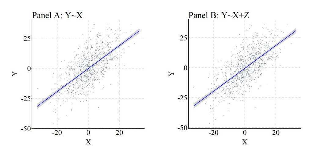
If you guessed “the estimated effects will slightly vary” you would be correct. You can see below that b = .95668 when Y was regressed on X, while b = .95673 when Y was regressed on X and Z. The slight differences in the estimates can be attributed to the existence of shared error due to the random variation used to specify the distribution of each construct. Alternatively, the estimated effects are essentially the same because only the variation that is shared between X, Y, and Z is removed from the calculation of the slope coefficient (b) for Y on X. That is, only a covariate that shares variation with both the independent and dependent variable will reduce the bias (when the covariate confounds the association of interest), misrepresent the effects (when the covariate mediates the association of interest), or increase the bias (when the covariate is a collider for the association of interest) observed in the estimated effects of the independent variable on the dependent variable.
> summary(lm(Y~X, data = Data))

Call:
lm(formula = Y ~ X, data = Data)

Residuals:
    Min      1Q  Median      3Q     Max
-38.598  -7.038  -0.491   6.679  33.637

Coefficients:
            Estimate Std. Error t value Pr(>|t|)
(Intercept) -0.19357    0.31959  -0.606    0.545
X            0.95668    0.03235  29.577   <2e-16 ***
---
Signif. codes:  0 ‘***’ 0.001 ‘**’ 0.01 ‘*’ 0.05 ‘.’ 0.1 ‘ ’ 1

Residual standard error: 10.09 on 998 degrees of freedom
Multiple R-squared:  0.4671,	Adjusted R-squared:  0.4666
F-statistic: 874.8 on 1 and 998 DF,  p-value: < 2.2e-16


> summary(lm(Y~X+Z, data = Data))

Call:
lm(formula = Y ~ X + Z, data = Data)

Residuals:
    Min      1Q  Median      3Q     Max
-38.911  -6.974  -0.603   6.564  33.727

Coefficients:
            Estimate Std. Error t value Pr(>|t|)
(Intercept) -0.19616    0.31962  -0.614    0.540
X            0.95673    0.03235  29.577   <2e-16 ***
Z           -0.03105    0.03274  -0.948    0.343
---
Signif. codes:  0 ‘***’ 0.001 ‘**’ 0.01 ‘*’ 0.05 ‘.’ 0.1 ‘ ’ 1

Residual standard error: 10.09 on 997 degrees of freedom
Multiple R-squared:  0.4676,	Adjusted R-squared:  0.4665
F-statistic: 437.8 on 2 and 997 DF,  p-value: < 2.2e-16
The similarities between the two models are illustrated in Figure 1, where the regression lines are almost identical.
[Figure 1]
Furthermore, to provide a comprehensive demonstration of this principle, we can replicate the simulation 10,000 times, randomly specify all of the key values – b, mean, and standard deviation –, and calculate the difference between the slope coefficient estimated when Y was regressed on X (i.e., M1_byx in the syntax) and the slope coefficient estimated when Y was regressed on X and Z (i.e., M2_byx in the syntax). As it can be observed, the difference between M1_byx and M2_byx – or D_byx – is extremely small at the 1st quartile, median, mean, and 3rd quartile, with only the minimum and maximum values demonstrating the existence of some deviation. These deviations, as discussed below, are likely the product of simulation anomalies.
> n<-10000
>
> set.seed(1992)
> Example1_DATA = foreach (i=1:n, .packages=c('lm.beta'), .combine=rbind) %dorng%
+   {
+     ### Value Specifications ####
+     N<-sample(150:10000, 1)
+     Z<-rnorm(N,runif(1,-5,5),runif(1,1,30))
+     X<-(runif(1,-10,10)*rnorm(N,runif(1,-5,5),runif(1,1,30)))
+     Y<-(runif(1,-10,10)*X)+(runif(1,-10,10)*rnorm(N,runif(1,-5,5),runif(1,1,30)))
+
+     Data<-data.frame(Z,X,Y)
+
+     ### Models ####
+     M1<-summary(lm(Y~X, data = Data))
+     M2<-summary(lm(Y~X+Z, data = Data))
+
+     M1_byx<-coef(M1)[2, 1]
+     M2_byx<-coef(M2)[2, 1]
+
+     D_byx<-M1_byx-M2_byx
+
+     # Data Frame ####
+
+     data.frame(i,N,M1_byx,M2_byx,D_byx)
+
+   }
>
> summary(Example1_DATA$D_byx)
           Min.         1st Qu.          Median            Mean         3rd Qu.            Max.
-1.759304446361 -0.000080997271 -0.000000297547 -0.000229557172  0.000073507961  0.782685990625
>
Non-Causally Associated Constructs: Covarying with Dependent Variable
Now, we have already reviewed that only the variation that is shared between X, Y,and Z is removed from the calculation of the slope coefficient (b), so if Z only shares variation with Y we can expect the same results as the previous simulation. We can simulate a non-causal correlation between two constructs by either (1) creating a construct that causes variation in both of the correlated constructs (i.e., a confounder) or by specifying shared residual variation. Personally, I prefer the former technique, but both techniques are extremely similar. In this simulation, we create a non-causal correlation between Z and Y by specifying that Cor – a normally distributed construct with a mean of 0 and standard deviation of 10 – causes variation in both Z and Y. When modeling the associations, let’s just forget Cor exists.
> ## Example ####
> n<-1000
>
> set.seed(1992)
>
> Cor<-rnorm(n,0,10)
> Z<-1*rnorm(n,0,10)+1*Cor
> X<-1*rnorm(n,0,10)
> Y<-1*X+1*rnorm(n,0,10)+1*Cor
>
> Data<-data.frame(Z,X,Y)
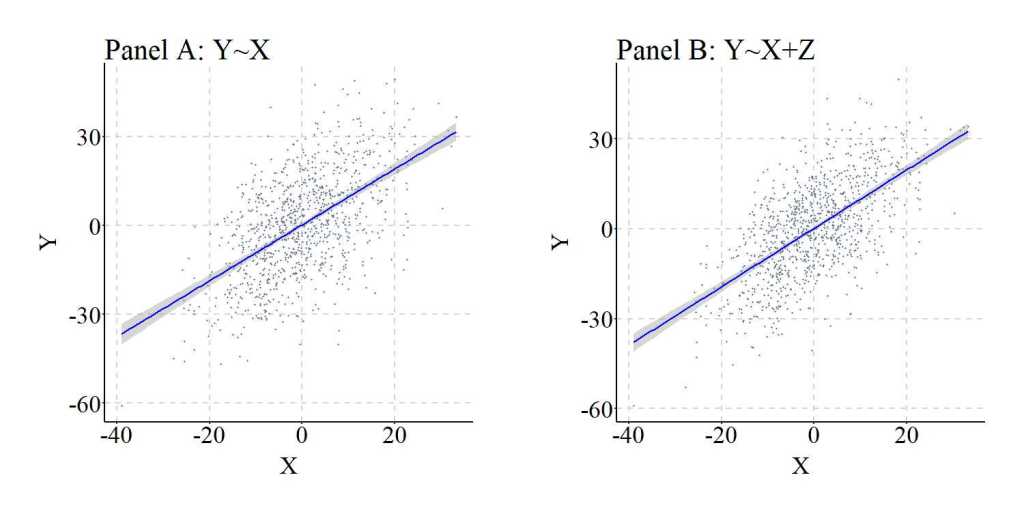
After simulating the data, we can estimate our models. Similar to the first simulation, the slope coefficient of the association between X and Y was .94287 when Z was not included in the model, and .97698 when Z was included as a covariate in the model. Again, the slight difference is the product of shared variation between X, Y, and Z.
> summary(lm(Y~X, data = Data))

Call:
lm(formula = Y ~ X, data = Data)

Residuals:
         Min           1Q       Median           3Q          Max
-47.55754362  -9.40598359   0.26206352   9.76044280  46.06588793

Coefficients:
               Estimate  Std. Error  t value             Pr(>|t|)
(Intercept) 0.265895531 0.446985198  0.59486              0.55207
X           0.942871210 0.044286559 21.29023 < 0.0000000000000002 ***
---
Signif. codes:  0 ‘***’ 0.001 ‘**’ 0.01 ‘*’ 0.05 ‘.’ 0.1 ‘ ’ 1

Residual standard error: 14.1316564 on 998 degrees of freedom
Multiple R-squared:  0.312328374,	Adjusted R-squared:  0.311639324
F-statistic:  453.27407 on 1 and 998 DF,  p-value: < 0.0000000000000002220446

>
> summary(lm(Y~X+Z, data = Data))

Call:
lm(formula = Y ~ X + Z, data = Data)

Residuals:
         Min           1Q       Median           3Q          Max
-40.23321543  -8.52102295   0.58367414   8.82508959  40.15749172

Coefficients:
                Estimate   Std. Error  t value             Pr(>|t|)
(Intercept) 0.0553391656 0.3936365735  0.14058              0.88823
X           0.9769833340 0.0390329312 25.02972 < 0.0000000000000002 ***
Z           0.4841391536 0.0283753707 17.06195 < 0.0000000000000002 ***
---
Signif. codes:  0 ‘***’ 0.001 ‘**’ 0.01 ‘*’ 0.05 ‘.’ 0.1 ‘ ’ 1

Residual standard error: 12.4388961 on 997 degrees of freedom
Multiple R-squared:  0.46774069,	Adjusted R-squared:  0.466672968
F-statistic: 438.073566 on 2 and 997 DF,  p-value: < 0.0000000000000002220446
Figure 2, similar to Figure 1, further illustrates the similarities between the results of the regression models.
[Figure 2]
Once again, replicating the simulation 10,000 times generally resulted in extremely small differences between the slope coefficient estimated when Y was regressed on X (i.e., M1_byx in the syntax) and the slope coefficient estimated when Y was regressed on X and Z (i.e., M2_byx in the syntax). Nevertheless, it is important to point out that the minimum difference between the slope coefficients was -209 and the maximum difference between the slope coefficients was 320. You might ask, why would differences that large occur? Well, to let you know the truth it is likely a simulation anomaly. That is, as the simulation is replicated and the values for the b, mean, and standard deviation are randomly sampled from uniform distributions, a perfect condition is sampled from the simulation space to create a statistical anomaly. Generally, these are rare, but occur at higher rates when the values for the b and standard deviation are selected from uniform distributions that have the ability to sample numbers close to 0. It is always important to consider the existence of anomalies when conducting simulations.
> n<-10000
>
> set.seed(1992)
> Example2_DATA = foreach (i=1:n, .packages=c('lm.beta'), .combine=rbind) %dorng%
+   {
+     ### Value Specifications ####
+     N<-sample(150:10000, 1)
+     Cor<-rnorm(N,runif(1,-5,5),runif(1,1,30))
+     Z<-(runif(1,-10,10)*rnorm(N,runif(1,-5,5),runif(1,1,30)))+(runif(1,-10,10)*Cor)
+     X<-(runif(1,-10,10)*rnorm(N,runif(1,-5,5),runif(1,1,30)))
+     Y<-(runif(1,-10,10)*X)+(runif(1,-10,10)*rnorm(N,runif(1,-5,5),runif(1,1,30)))+(runif(1,-10,10)*Cor)
+
+     Data<-data.frame(Z,X,Y)
+
+     ### Models ####
+     M1<-summary(lm(Y~X, data = Data))
+     M2<-summary(lm(Y~X+Z, data = Data))
+
+     M1_byx<-coef(M1)[2, 1]
+     M2_byx<-coef(M2)[2, 1]
+
+     D_byx<-M1_byx-M2_byx
+
+     # Data Frame ####
+
+     data.frame(i,N,M1_byx,M2_byx,D_byx)
+
+   }
>
> summary(Example2_DATA$D_byx)
          Min.        1st Qu.         Median           Mean        3rd Qu.           Max.
-209.741442187   -0.005051558   -0.000004274   -0.013072247    0.004472406  320.331011725
Non-Causally Associated Constructs: Covarying with Independent Variable
Let’s finish up this section by exploring the effects of a non-causal correlation between Z and X. Following the previous simulation, we create a non-causal correlation between Z and X by specifying that Cor – a normally distributed construct with a mean of 0 and standard deviation of 10 – causes variation in both Z and X.
> n<-1000
>
> set.seed(1992)
>
> Cor<-rnorm(n,0,10)
> Z<-1*rnorm(n,0,10)+1*Cor
> X<-1*rnorm(n,0,10)+1*Cor
> Y<-1*X+1*rnorm(n,0,10)
>
> Data<-data.frame(Z,X,Y)
>
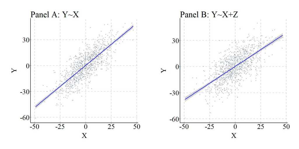
Evident by the results of the models, the slope coefficient of the association between X and Y was .97509 when Z was not included in the model, and .97368 when Z was included as a covariate in the model. Again, the slight difference is the product of shared variation between X, Y, and Z.
> summary(lm(Y~X, data = Data))

Call:
lm(formula = Y ~ X, data = Data)

Residuals:
         Min           1Q       Median           3Q          Max
-32.64604854  -6.56097850   0.28267451   6.70606963  39.12979940

Coefficients:
               Estimate  Std. Error  t value             Pr(>|t|)
(Intercept) 0.353333856 0.329484762  1.07238              0.28381
X           0.975090101 0.023839719 40.90191 < 0.0000000000000002 ***
---
Signif. codes:  0 ‘***’ 0.001 ‘**’ 0.01 ‘*’ 0.05 ‘.’ 0.1 ‘ ’ 1

Residual standard error: 10.4167819 on 998 degrees of freedom
Multiple R-squared:  0.626352477,	Adjusted R-squared:  0.62597808
F-statistic: 1672.96645 on 1 and 998 DF,  p-value: < 0.0000000000000002220446

>
> summary(lm(Y~X+Z, data = Data))

Call:
lm(formula = Y ~ X + Z, data = Data)

Residuals:
         Min           1Q       Median           3Q          Max
-32.60805564  -6.55249618   0.26957028   6.73053562  39.13236765

Coefficients:
                 Estimate    Std. Error  t value             Pr(>|t|)
(Intercept) 0.35153822414 0.33002211971  1.06520              0.28705
X           0.97368272558 0.02684369244 36.27231 < 0.0000000000000002 ***
Z           0.00305349263 0.02672169109  0.11427              0.90905
---
Signif. codes:  0 ‘***’ 0.001 ‘**’ 0.01 ‘*’ 0.05 ‘.’ 0.1 ‘ ’ 1

Residual standard error: 10.4219364 on 997 degrees of freedom
Multiple R-squared:  0.62635737,	Adjusted R-squared:  0.625607836
F-statistic:  835.66254 on 2 and 997 DF,  p-value: < 0.0000000000000002220446
To illustrate the similarities between the results of the regression models, Figure 3 was produced.
[Figure 3]
We again can replicate the simulation 10,000 times, randomly specify all of the key values – b, mean, and standard deviation –,and calculate the difference between the slope coefficient estimated when Y was regressed on X (i.e., M1_byx in the syntax) and the slope coefficient estimated when Y was regressed on X and Z (i.e., M2_byx in the syntax). As it can be observed, the difference between M1_byx and M2_byx – or D_byx – is extremely small at the 1st quartile, median, mean, and 3rd quartile, with only the minimum and maximum values demonstrating the existence of some deviation. These deviations, again, are likely the product of simulation anomalies.
> n<-10000
>
> set.seed(1992)
> Example3_DATA = foreach (i=1:n, .packages=c('lm.beta'), .combine=rbind) %dorng%
+   {
+     ### Value Specifications ####
+     N<-sample(150:10000, 1)
+     Cor<-rnorm(N,runif(1,-5,5),runif(1,1,30))
+     Z<-(runif(1,-10,10)*rnorm(N,runif(1,-5,5),runif(1,1,30)))+(runif(1,-10,10)*Cor)
+     X<-(runif(1,-10,10)*rnorm(N,runif(1,-5,5),runif(1,1,30)))+(runif(1,-10,10)*Cor)
+     Y<-(runif(1,-10,10)*X)+(runif(1,-10,10)*rnorm(N,runif(1,-5,5),runif(1,1,30)))
+
+     Data<-data.frame(Z,X,Y)
+
+     ### Models ####
+     M1<-summary(lm(Y~X, data = Data))
+     M2<-summary(lm(Y~X+Z, data = Data))
+
+     M1_byx<-coef(M1)[2, 1]
+     M2_byx<-coef(M2)[2, 1]
+
+     D_byx<-M1_byx-M2_byx
+
+     # Data Frame ####
+
+     data.frame(i,N,M1_byx,M2_byx,D_byx)
+
+   }
>
> summary(Example3_DATA$D_byx)
           Min.         1st Qu.          Median            Mean         3rd Qu.            Max.
-2.389818583275 -0.001469675403 -0.000000033681 -0.000511453956  0.001380548570  1.467722891503
Discussion
As demonstrated by the results, adjusting for the variation in a construct correlated with neither or one of the constructs of interest will have limited impact on the estimated slope coefficient. That is, if Z does not share variation with both X and Y, the slope coefficient of the association between X and Y will not become biased by excluding Z in the estimated regression model. Although the simulations reviewed above do not demonstrate a source of statistical bias, it does demonstrate that adjusting for a variable that does not share variation with both X and Y has limited impact on the estimated effects of X on Y. As such, for the sake of parsimony, it is best we exclude constructs from our regression models that do not covary with both the independent and dependent variables of interest.
Now let’s take a brief intermission and then move onto the second topic of this entry: misspecified causal structure.
Intermission: Theoretical Discussion of Bivariate and Multivariable Regression Models
Okay, so this is not much of an intermission, but I really wanted to have a theoretical discussion about multivariable regression models at some point in the Statistical Biases when Examining Causal Associations section. So here we are…
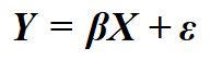
Let me start off by stating this, when we estimate a bivariate regression model we are intrinsically stating that we believe that variation in X (or the identified independent variable) causes variation in Y (or the identified dependent variable). Here, I am using cause to mean either a direct or indirect cause. This intrinsic statement exists for a variety of reasons, the primary being that your bivariate regression model is a directed equation from X to Y. That is, Equation 1 is equal to Figure 4.
[Equation 1]
[Figure 4]
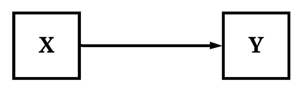
It is easy to consider this an overstatement, but when have we ever estimated a regression equation with an independent variable that was believed to not cause variation in the dependent variable. I for one have never been shocked when the slope coefficient produced by a model suggests a meaningful effect of the independent variable on the dependent variable. I, however, have experienced that feeling when the resulting model coefficients suggest that an association does not exist between the independent variable and the dependent variable. These feelings occur because our prior knowledge and experiences informs the hypotheses we develop about how the universe works and, in turn, guide the specification of our regression models. If you still disagree, consider the research published or grant applications. Often they are relatively straight forward research questions, like incarceration influences employment. Or an empirical evaluation of a theoretical model of how the universe works. Or a grant to help an agency implement evidence based training in hopes that it causes positive change in the clienteles’ lives.
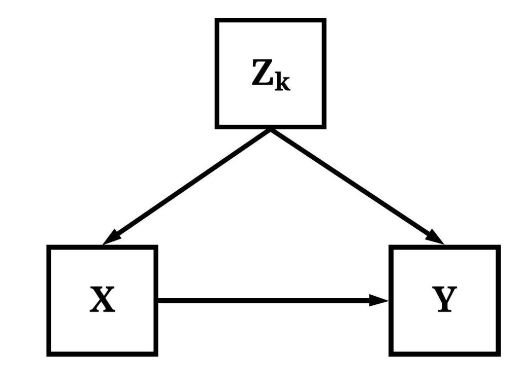
If Equation 1 intrinsically expresses our belief that variation in X causes variation in Y – i.e., a causal statement of how the world works –, what does Equation 2 express? Following the same logic, the inclusion of a covariate inherently expresses the believe that variation in Zk (i.e., covariates) causes variation in both X and Y. Specifically, the inclusion of any Zk expresses that we believe the association between X and Y can not be properly estimated without adjusting for the variation associated with Zk. Here, Equation 2 is equivalent to Figure 5.
[Equation 2]
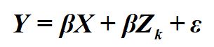
[Figure 5]
Now, you might be asking, why is it important for us to acknowledge that a regression equation is inherently an expression of causal beliefs? At the forefront, acknowledging the underlying causal expression of a regression equation increases our care when estimating a multivariable model. That is, by acknowledging that Equation 2 represents the belief that Zk (i.e., covariates) cause variation in both X and Y, we can be more careful about the covariates that are included in our equations. Only constructs that are believed to cause variation in both X and Y, or as covered in Entry 10 is a descendant of a construct that causes variation in both X and Y, should be included in a multivariable regression model. Everything else need not be included as additional covariates because they can: (1) reduce the degrees of freedom, (2) introduce bias or misrepresent the causal association between constructs, (3) have limited influence on estimating the causal effects of X on Y, and (4) increase the likelihood of overfitting a model. In the end, recognizing our causal claims within our statistics can only serve to benefit the advancement of our knowledge.
I apologize for getting on my high horse but I do believe this is extremely important. Being careful with statistics is important as we are making causal claims about how the world works within our equations.
Now, let’s talk about misspecifying the causal structure in a regression model!
Misspecified Causal Structure: Reverse Causal Specification
Considering our intermission discussion, if a regression equation is inherently a statement of causal processes, the specification of our regression model will either (1) capture the correct causal pathway from one variable to another variable or (2) misspecify the causal pathway from one variable to another variable. The latter is much more likely, hence the discussions dedicated to Colliders, Confounders, Descendants, and Mediators/ Moderators. But there is one more misspecification that we might include in a regression model, the reverse causal specification. As implied, the reverse causal specification refers to the condition where we flip the two constructs in the equation and estimate the effects of the true dependent construct (i.e., the construct where variation is being caused) on the true independent construct (i.e., the construct causing variation). To provide an easy example, we can estimate the effects of college major on career employment or career employment on college major. The first regression model will produce estimates capturing the causal effects, while the second regression model will produce estimates capturing the reverse effects. In this example, we are assuming that the measurement of college major only captures the first attempt at college.
While it is easy to recognize that the second regression model in the example above implies the reverse causal specification, it is extremely difficult in practice to identify reverse causal specifications in cross-sectional data. For example, did marijuana smoking cause an individual to express symptoms of depression or did symptoms of depression cause an individual to smoke marijuana? If both constructs are measured at the same time period, it is difficult to discern and estimate the causal effects of one on the other. Furthermore, we condition the statement with “cross-sectional data” because causal effects can not work backwards in time and longitudinal methods permit the estimation of simultaneous regression models to examine reciprocal associations. Given this, the likelihood of estimating a regression model with the reverse causal specification is substantially higher when employing cross-sectional data. Independent of the data structure, estimating a regression model with the reverse causal specification can produce findings supportive of the misspecified causal structure. To demonstrate, let’s again conduct a data simulation.
For this data simulation, we are going to simply use a bivariate directed equation specification to simulate the causal effects of X on Y. X, following the simulations above, is a normally distributed construct with a mean of 0 and a standard deviation of 10, where a 1 point increase in X causes a 1 point increase in Y. The residual variation in Y is normally distributed with a mean of 0 and a standard deviation of 10.
> ## Example ####
> n<-1000
>
> set.seed(1992)
>
> X<-1*rnorm(n,0,10)
> Y<-1*X+1*rnorm(n,0,10)
>
> Data<-data.frame(X,Y)
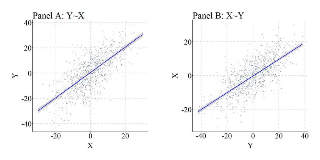
After simulating the data, we can regress Y on X and X on Y and observe the slope coefficients produced by the OLS models. Evident by the findings, regressing Y on X suggests that a 1 point increase in X causes a 1.002 point increase in Y, which is consistent with the specification of the data simulation. Alternatively, regressing X on Y suggests that a 1 point increase in Y causes a .4939 increase in X, suggesting the existence of a reciprocal causal pathway. This reciprocal causal pathway, however, does not exist as our simulation specification dictated that the variation in Y was the product of the variation in X, and not vice versa.
> summary(lm(Y~X, data = Data))

Call:
lm(formula = Y ~ X, data = Data)

Residuals:
         Min           1Q       Median           3Q          Max
-33.39823634  -6.39223268  -0.12454071   6.77441730  32.32615833

Coefficients:
                Estimate   Std. Error  t value             Pr(>|t|)
(Intercept) 0.5328217473 0.3123247274  1.70599             0.088322 .
X           1.0016311375 0.0320395916 31.26229 < 0.0000000000000002 ***
---
Signif. codes:  0 ‘***’ 0.001 ‘**’ 0.01 ‘*’ 0.05 ‘.’ 0.1 ‘ ’ 1

Residual standard error: 9.87622125 on 998 degrees of freedom
Multiple R-squared:  0.494768228,	Adjusted R-squared:  0.494261984
F-statistic: 977.331038 on 1 and 998 DF,  p-value: < 0.0000000000000002220446

>
> summary(lm(X~Y, data = Data))

Call:
lm(formula = X ~ Y, data = Data)

Residuals:
          Min            1Q        Median            3Q           Max
-22.946438389  -4.195328463  -0.078404385   4.594062381  22.235582859

Coefficients:
                 Estimate    Std. Error  t value             Pr(>|t|)
(Intercept) -0.3048824723  0.2194381704 -1.38938              0.16503
Y            0.4939625074  0.0158005841 31.26229 < 0.0000000000000002 ***
---
Signif. codes:  0 ‘***’ 0.001 ‘**’ 0.01 ‘*’ 0.05 ‘.’ 0.1 ‘ ’ 1

Residual standard error: 6.93559772 on 998 degrees of freedom
Multiple R-squared:  0.494768228,	Adjusted R-squared:  0.494261984
F-statistic: 977.331038 on 1 and 998 DF,  p-value: < 0.0000000000000002220446

>
Although the lines appear to be identical, it is important to note that the x and y-axes switch from Panel A to Panel B. Notably, independent of the exact slope coefficients, the results in Figure 6 further solidify the suggestion that variation in X causes variation in Y and variation in Y causes variation in X. This interpretation, however, is incorrect as it does not align with the simulation specification.
[Figure 6]
You might be asking, how often can the reverse specification produce results supporting the reciprocal causal pathway? Well it is all conditional upon the true causal effects of X on Y. Specifically, the likelihood of observing results supporting the reciprocal causal pathway is diminished if the variation in X has a weak (relative to the scale of the constructs) causal influence on the variation in Y, while the likelihood of observing results supporting the reciprocal causal pathway is increased if the variation in X has a strong (relative to the scale of the constructs) causal influence on the variation in Y. Given that the reverse causal pathway is conditional upon the specified causal effects of X on Y, it is extremely difficult to discern a rate at which this can happen. Coinciding with this difficulty, we will not conduct replications of the simulation because the resulting information could misguide or be misinterpreted as evidence of the rate at which the results from a misspecified regression model supports the reciprocal causal pathway.
Conclusion
Overall, I believe this entry represents a perfect end to our first simulated exploration of the statistical biases that could exist when examining causal associations. As reviewed, a construct correlated with neither or either the independent or dependent variable produces limited biases when estimating the association of interest. Moreover, as discussed in the second half of this entry, the estimation of a regression model with the reverse causal specification using cross-sectional data could provide evidence supporting the existence of a reciprocal causal pathway. Although relatively straightforward, it is important to consider this when identifying and estimating the causal pathway from one construct to another construct. Now, let’s move on to examining the statistical biases that could be generated by factors related to measurement!
[i] This is a theme that will continue until the end of the Sources of Statistical Biases Series! There will always be issues and topics to revisit!
[ii] For a great depiction of the latter situation, simply review Tyler Vigen’s seminal work on spurious correlations (http://www.tylervigen.com/spurious-correlations). I think my favorite is the number of people who drowned in a pool and the number of films Nicholas Cage appeared in each year, which has a correlation of (r = .66). The observed correlation is likely the product of measurement error – I can’t think of any thing that could be a common cause –, but you never know…
[iii] I do like the idea of a computer programming employment opportunity for incarcerated individuals, but a lot of kinks would have to be worked out.
License: Creative Commons Attribution 4.0 International (CC By 4.0)
