Generating causal inferences is a difficult process. We can run a true experiment (i.e., a randomized controlled trial), however that can be ethically concerning when randomizing certain treatments. Alternatively, we can develop a Directed Acyclic Graph (DAG) and reduce the influence of confounders and colliders on our association of interest. Or we can conduct complex statistical analyses, such as a regression discontinuity model, a difference-in-difference model, or a lagged panel model. Nevertheless, these techniques are subject to various assumptions – discussions planned in the future – and might not be applicable for the association of interest. As such, we might have to rely on an alternative approach for generating causal inferences: instrumental variable analysis.
Instrumental Variables
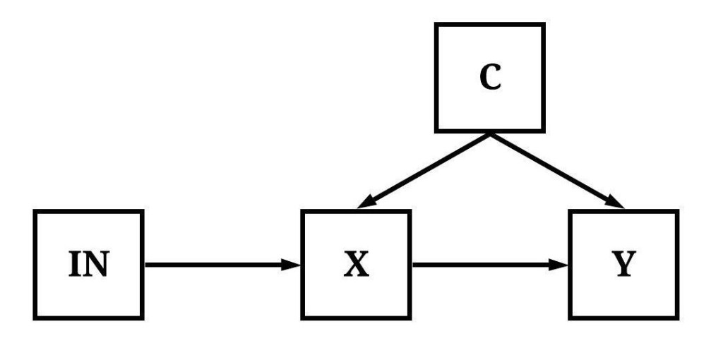
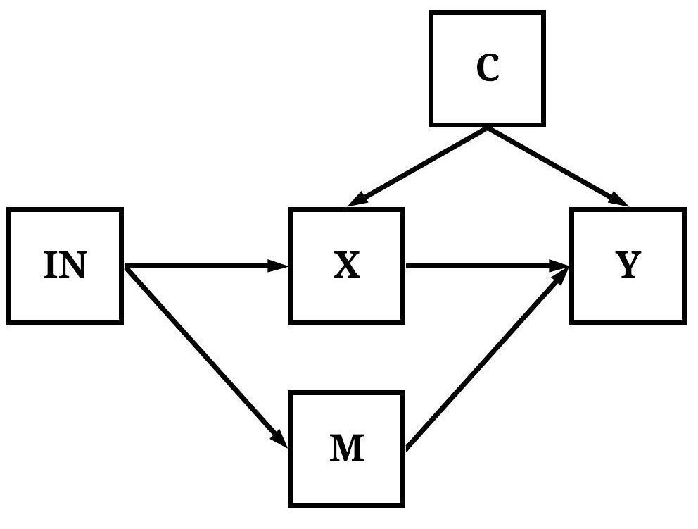
Let’s take a moment to define instrumental variables and identify constructs that can be categorized as instruments. A construct can be employed as an instrument when: (1) the variation in the construct directly causes variation in the independent variable, (2) the variation in a construct is uncorrelated with any confounders, (3) the variation in the construct does not directly cause variation in the dependent variable, and (4) the variation in the construct does not have any other indirect causal influence on the dependent variable (Figure 1). As illustrated below, IN satisfies these requirements, making it an instrument for the association between X and Y, which permits the estimation of an instrumental variable analysis.
[Figure 1]
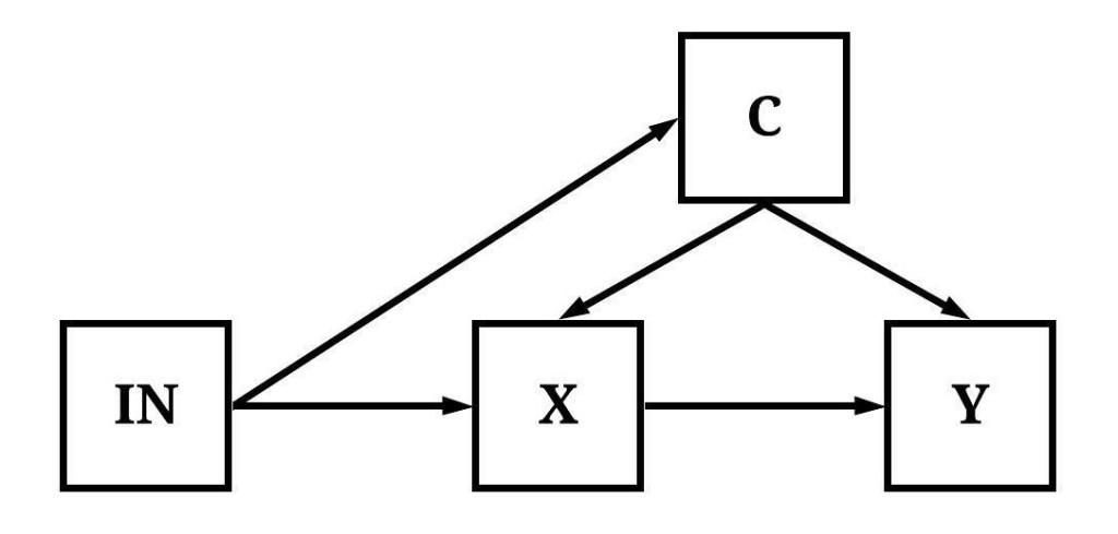
In figures 2-5, IN would not qualify as an instrumental variable. Explicitly, in Figure 2, IN has an indirect effect on X and Y through C.
[Figure 2]
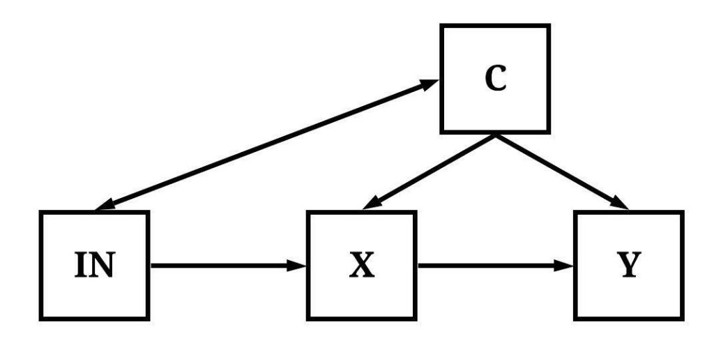
In Figure 3, the variation in IN is correlated with the variation in C.
[Figure 3]
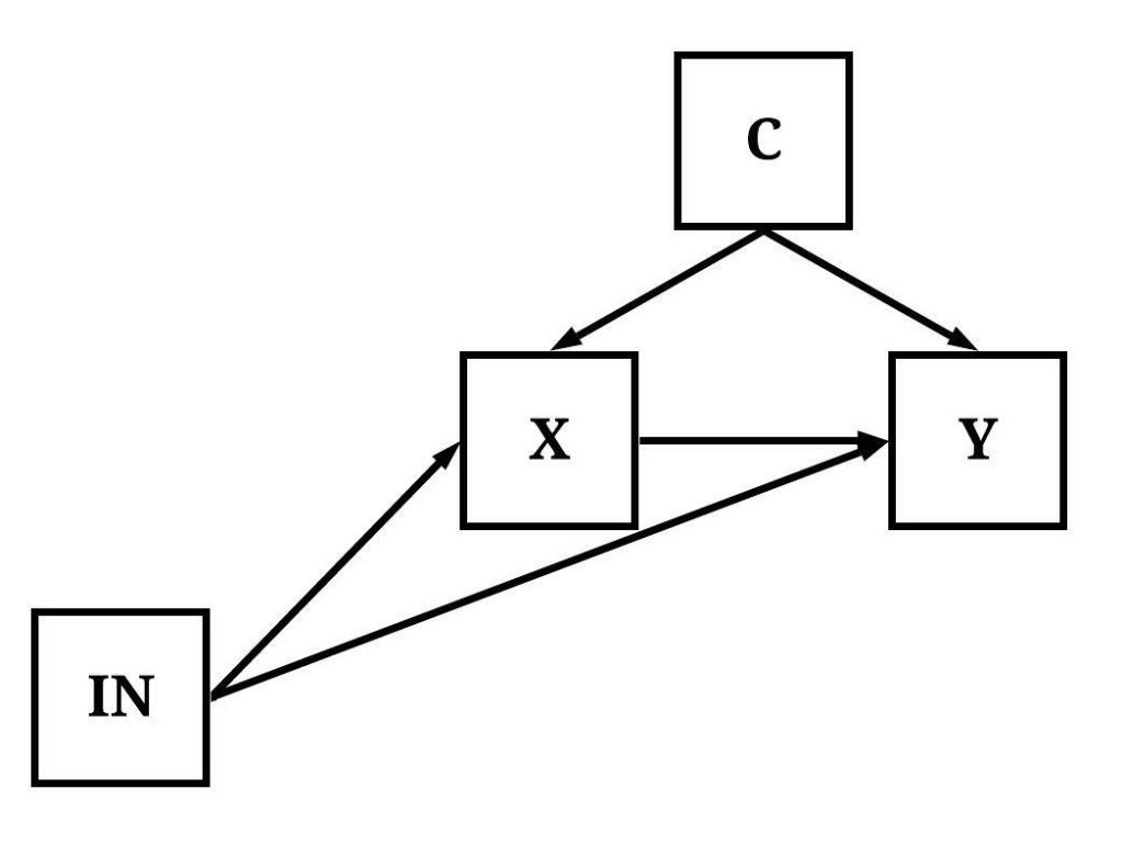
In Figure 4, variation in IN has a direct causal effect on both the variation in X and the variation in Y.
[Figure 4]
In Figure 5, variation in IN causally influences variation in Y indirectly through both X and M.
[Figure 5]
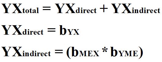
As one can recognized, it is quite difficult to identify a construct that satisfies the requirements of an instrumental variable. These requirements, however, serve a valuable purpose when trying to generate causal inferences about the effects of X on Y. In particular, by finding the perfect instrument, one can estimate the causal effects of X on Y (bYX) without observing the known or unknown mechanisms confounding the association. To demonstrate how instrumental variable analysis works, let’s briefly review how to calculate the total, direct, and indirect effects of one construct on another construct. As presented in Equation 1, the total effect of X on Y is equal to the direct effect (bYX) of X on Y plus the indirect effect of X on Y (bMEX*bYME). The indirect effect is calculated as the effects of X on the mediator (ME) multiplied by the effects of the mediator (ME) on Y.
[Equation 1]
Translating this to an instrumental variable analysis, we can replace X with IN.
[Equation 2]
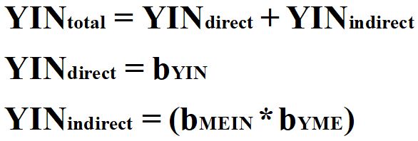
Now that we have translated the equation for Y and IN, we can observe how the requirements of an instrument can permit the observation of the causal effects of X on Y. First, as identified above, the instrument can not have a direct influence on Y. By satisfying this requirement, we can remove the direct effects portion of the equation because bYIN is assumed to be equal to 0.
[Equation 3]
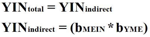
Second, the instrumental variable can not have any other indirect causal influence on the dependent variable. By satisfying this requirement, we can set the indirect equation to only represent the indirect pathway through the independent construct of interest (X).
[Equation 4]
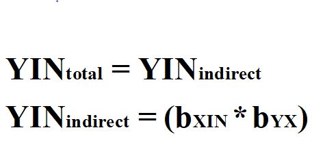
Third, the variation in the instrumental variable is required to be uncorrelated with any mechanisms that confound the association of interest. By satisfying this requirement, the total effects of IN on Y– bYIN– will remain unbiased. Equation 4 represents the calculation of the total effects of IN on Y when a construct satisfies the requirements for being designated as an instrumental variable.
[Equation 5]

Through reverse estimation, we can solve Equation 4 to identify the causal effects of X on Y (bYX). The reverse estimation can be done by: (1) regressing Y on IN to observe the slope coefficient representative of the total effects of IN on Y and (2) regressing X on IN to observe the slope coefficient representative of the direct effects of IN on X. After estimating these regression models, we can solve for bYX by setting bYX equal to bYIN divided by bXIN.
[Equation 6]
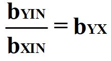
To provide an example, if the slope coefficient of the total effects of Y on IN is equal to 1 and the slope coefficient of the IN on X is equal to 2, bYX is equal to .50 even if the association between X and Y is confounded by C. But let’s work through some simulations!
An Appropriate Instrument
Using the diagram presented in Figure 1, we can simulate a structural system with an association between X and Y, where variation in X is causally influenced by variation in the instrumental variable (IN) and a confounder (C) and the variation in Y is causally influenced by the variation in X and the confounder (C). For simplicity, the distribution of scores on the confounder (C) and the instrumental variable (IN) were specified to have a mean of 0 and a standard deviation of 10, while the residual variation for X and Y was specified to have a mean of 0 and a standard deviation of 10. The slope coefficient of C and IN on X was set equal to 1, while the slope coefficient of C and X on Y was set equal to 1.
> ## Example 1 ####
> n<-1000
>
> set.seed(1992)
>
> C<-rnorm(n,0,10)
> IN<-rnorm(n,0,10)
> X<-1*C+1*IN+1*rnorm(n,0,10)
> Y<-1*C+1*X+1*rnorm(n,0,10)
After simulating the data, we can estimate the confounded and unconfounded association between X and Y. Evident by the estimates, the confounded slope coefficient was bYX=1.313 and the slope coefficient produced by the model adjusting for the influence of C was bYX=.986. This demonstrates that not adjusting for C in the regression equation produces confounder bias when estimating the effects of X on Y.
# Confounded Model ###
> summary(lm(Y~X))

Call:
lm(formula = Y ~ X)

Residuals:
         Min           1Q       Median           3Q          Max
-42.48178035  -8.95502545   0.05464166   9.34051095  42.09044496

Coefficients:
                Estimate   Std. Error  t value             Pr(>|t|)
(Intercept) 0.2052258593 0.4154580586  0.49397              0.62143
X           1.3127961362 0.0248194464 52.89385 < 0.0000000000000002 ***
---
Signif. codes:  0 ‘***’ 0.001 ‘**’ 0.01 ‘*’ 0.05 ‘.’ 0.1 ‘ ’ 1

Residual standard error: 13.1366588 on 998 degrees of freedom
Multiple R-squared:  0.737075026,	Adjusted R-squared:  0.736811574
F-statistic: 2797.75962 on 1 and 998 DF,  p-value: < 0.0000000000000002220446

> lm.beta(lm(Y~X))

Call:
lm(formula = Y ~ X)

Standardized Coefficients::
   (Intercept)              X
0.000000000000 0.858530736884

# Unconfounded Model ###
>
> summary(lm(Y~X+C))

Call:
lm(formula = Y ~ X + C)

Residuals:
         Min           1Q       Median           3Q          Max
-32.87338972  -6.48966902   0.36362255   6.78372717  39.13992447

Coefficients:
                Estimate   Std. Error  t value             Pr(>|t|)
(Intercept) 0.3636575998 0.3297320015  1.10289              0.27034
X           0.9855920916 0.0238734227 41.28407 < 0.0000000000000002 ***
C           0.9940259708 0.0409924314 24.24901 < 0.0000000000000002 ***
---
Signif. codes:  0 ‘***’ 0.001 ‘**’ 0.01 ‘*’ 0.05 ‘.’ 0.1 ‘ ’ 1

Residual standard error: 10.4239797 on 997 degrees of freedom
Multiple R-squared:  0.834615908,	Adjusted R-squared:  0.834284145
F-statistic: 2515.69559 on 2 and 997 DF,  p-value: < 0.0000000000000002220446

> lm.beta(lm(Y~X+C))

Call:
lm(formula = Y ~ X + C)

Standardized Coefficients::
   (Intercept)              X              C
0.000000000000 0.644548747046 0.378588396674

>
Now let’s turn our attention to the instrumental variable analysis by regressing Y on IN and X on IN. The slope coefficient produced by the model regressing Y on the instrumental variable was bYIN=.962 and the slope coefficient produced by the model regressing X on the instrumental variable was bXIN=.958. Using the calculation above, we can estimate that the causal effects of X on Y is equal to approximately bYX = 1.004, which is close to the specification of the simulated data (bYX= 1.000) and approximately .018 larger than the slope coefficient produced by the unconfounded model.
> # Y on Instrumental Variable ###
> summary(lm(Y~IN))

Call:
lm(formula = Y ~ IN)

Residuals:
         Min           1Q       Median           3Q          Max
-70.73574803 -17.40492518   1.02465114  16.11752345  75.55079914

Coefficients:
                   Estimate      Std. Error  t value             Pr(>|t|)
(Intercept) -0.000430986651  0.753532943015 -0.00057              0.99954
IN           0.961597210437  0.076262940367 12.60897 < 0.0000000000000002 ***
---
Signif. codes:  0 ‘***’ 0.001 ‘**’ 0.01 ‘*’ 0.05 ‘.’ 0.1 ‘ ’ 1

Residual standard error: 23.7941498 on 998 degrees of freedom
Multiple R-squared:  0.137414049,	Adjusted R-squared:  0.136549735
F-statistic: 158.986152 on 1 and 998 DF,  p-value: < 0.0000000000000002220446

> lm.beta(lm(Y~IN))

Call:
lm(formula = Y ~ IN)

Standardized Coefficients::
   (Intercept)             IN
0.000000000000 0.370694010171

>
> # X on Instrumental Variable ###
> summary(lm(X~IN))

Call:
lm(formula = X ~ IN)

Residuals:
         Min           1Q       Median           3Q          Max
-48.69473518  -9.55124948  -0.46506143   9.14557423  46.89763854

Coefficients:
                 Estimate    Std. Error  t value            Pr(>|t|)
(Intercept) -0.2769319073  0.4378308474 -0.63251              0.5272
IN           0.9582718965  0.0443116232 21.62575 <0.0000000000000002 ***
---
Signif. codes:  0 ‘***’ 0.001 ‘**’ 0.01 ‘*’ 0.05 ‘.’ 0.1 ‘ ’ 1

Residual standard error: 13.8252917 on 998 degrees of freedom
Multiple R-squared:  0.319084078,	Adjusted R-squared:  0.318401798
F-statistic:  467.67288 on 1 and 998 DF,  p-value: < 0.0000000000000002220446

> lm.beta(lm(X~IN))

Call:
lm(formula = X ~ IN)

Standardized Coefficients::
   (Intercept)             IN
0.000000000000 0.564875276591

>
You might be asking why are their slight differences for the bYX between the instrumental variable analysis, the unconfounded model, and the simulation specification. These slight differences exist because we can not generate random variables that are perfectly uncorrelated. For example, a slight non-causal correlation exists between the confounder and the instrumental variable due to the random selection of scores from a uniform distribution. However, as demonstrated above, an instrumental variable analysis provides the ability to deduce the causal effects of one construct on another construct when (1) the association of interest is confounded by unobserved mechanisms and (2) when the instrument satisfies the requirements of an instrumental variable analysis.
> # Test ###
> cor(IN,C)
[1] 0.00161152766817
However, let’s replicate this analysis 50,000 with random estimates to demonstrate the average distance between the slope coefficient produced by the instrumental variable analysis and the slope coefficient produced by the unconfounded model. The syntax below was used to conduct the randomly specified simulation analysis.
## Replicated Example 1 ####
n<-50000

set.seed(1992)
Example1_DATA = foreach (i=1:n, .packages=c('lm.beta'), .combine=rbind) %dorng%
  {
    ### Value Specifications ####
    ## Example 1 ####
    N<-sample(150:10000, 1)

    set.seed(1992)

    Con<-(rnorm(N,runif(1,-5,5),runif(1,1,30)))
    IN<-(rnorm(N,runif(1,-5,5),runif(1,1,30)))
    X<-(runif(1,.1,10))*Con+(runif(1,.1,10))*IN+(runif(1,.1,10))*(rnorm(N,runif(1,-5,5),runif(1,1,30)))
    Y<-(runif(1,.1,10))*Con+(runif(1,.1,10))*X+(runif(1,.1,10))*(rnorm(N,runif(1,-5,5),runif(1,1,30)))


    ### Models
    M1<-summary(lm(Y~X+Con))
    M2<-summary(lm(Y~IN))
    M3<-summary(lm(X~IN))

    M1_byx<-coef(M1)[2, 1]
    M2_byin<-coef(M2)[2, 1]
    M3_bxin<-coef(M3)[2, 1]

    IN_byx<-M2_byin/M3_bxin

    # Data Frame ####

    data.frame(i,N,M1_byx,M2_byin,M3_bxin,IN_byx)

  }
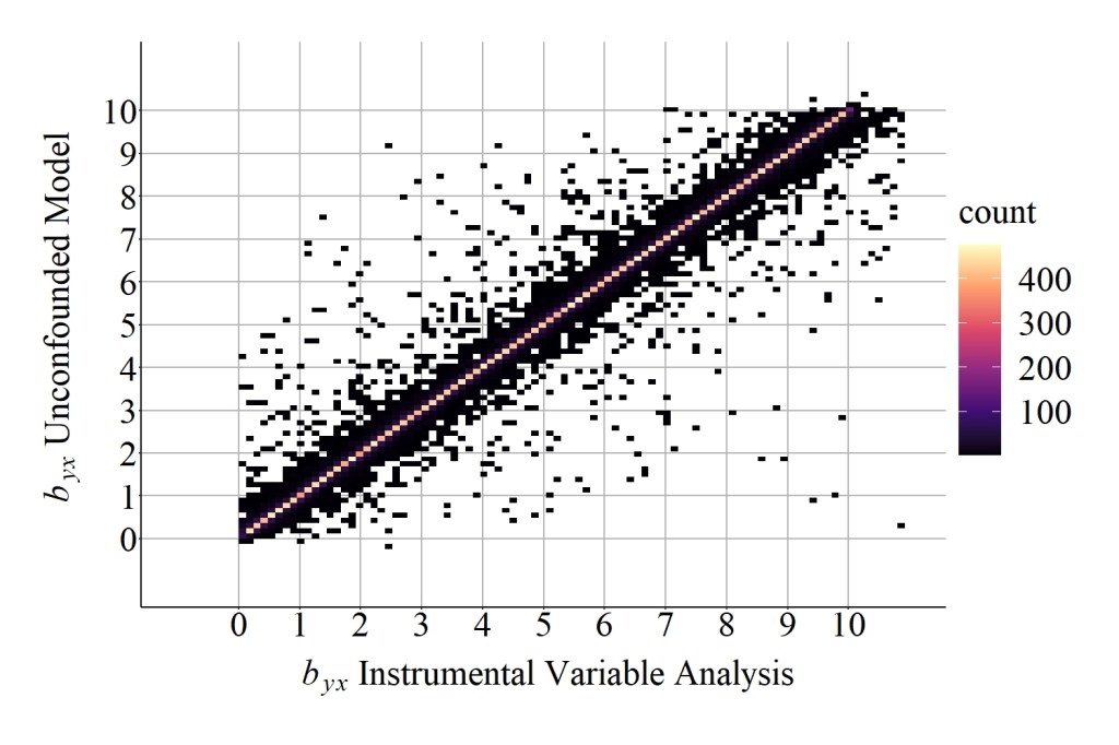
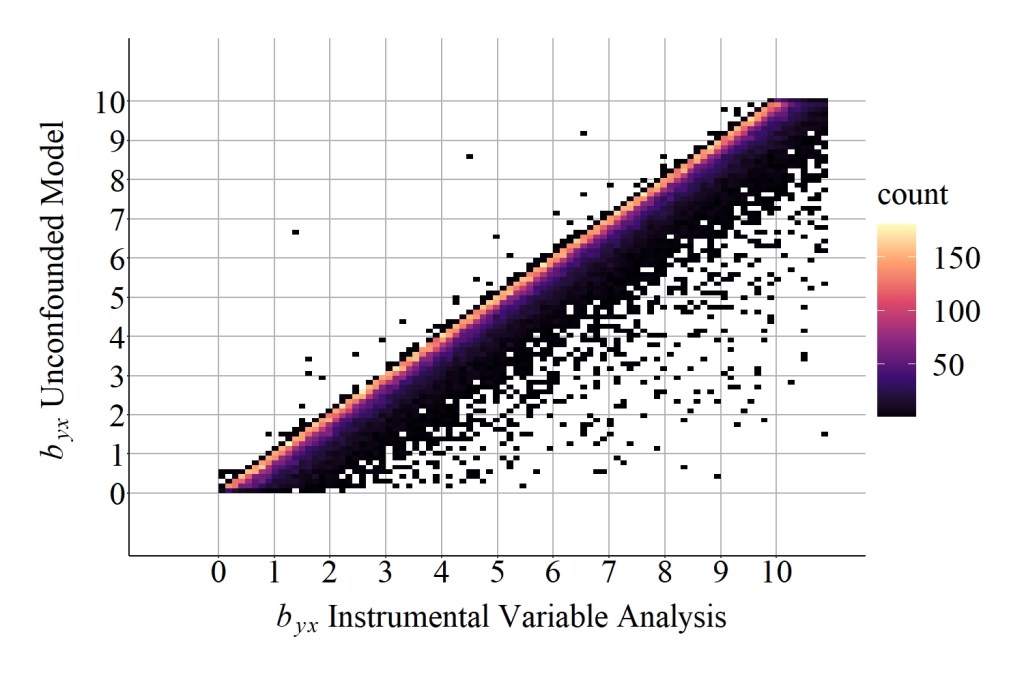
As demonstrated in Figure 6, the slope coefficient for the association between X and Y produced by the unconfounded model has almost a perfect positive correlation with the slope coefficient produced by the instrumental variable analysis across the 50,000 randomly specified simulations. To be precise, the correlation is .93 after removing 291 simulations due to the production of simulation anomalies. Moreover, the median difference between the slope coefficient produced by the unconfounded model and the slope coefficient produced by the instrumental variable analysis was 0.0000969833, while the mean difference was 0.0248374101. Altogether, the randomly specified simulation analysis provides evidence supporting the validity of the instrumental variable approach and demonstrates that instrumental variables can be used to estimate the causal effects of X on Y.
> corr.test(DF$IN_byx,DF$M1_byx)
Call:corr.test(x = DF$IN_byx, y = DF$M1_byx)
Correlation matrix
[1] 0.93
Sample Size
[1] 49799
These are the unadjusted probability values.
  The probability values  adjusted for multiple tests are in the p.adj object.
[1] 0

 To see confidence intervals of the correlations, print with the short=FALSE option
>
> summary(DF$IN_byx-DF$M1_byx)
          Min.        1st Qu.         Median           Mean        3rd Qu.           Max.
 -6.7471599646  -0.0137575791   0.0000969833   0.0248374101   0.0151523267 121.1289942258
>
[Figure 6]
But let’s be honest… you did not read this entry because you were worried about the validity of an instrumental variable analysis. You came here because you want to see what happens when we mis-identify an instrumental variable. That is, you want to see the bias that exists when we include one of the instruments in figures 2-5 in our analysis! Don’t worry I do too! Although not exhaustive, we will continue our discussion by conducting four randomly specified simulation analyses.
Misidentified Instrument: IN causes variation in C
Using the diagram presented in Figure 2, an updated simulation analysis was conducted where variation in the instrumental variable (IN) caused variation in the confounder (C). Identical to the previous simulation analysis, 50,000 randomly specified simulations were estimated and the slope coefficients for the causal effects of X on Y (bYX) produced by the unconfounded model and the instrumental variable models were compared.
> n<-50000
>
> set.seed(1992)
> Example2_DATA = foreach (i=1:n, .packages=c('lm.beta'), .combine=rbind) %dorng%
+   {
+     ### Value Specifications ####
+     ## Example 2 ####
+     N<-sample(150:10000, 1)
+
+     IN<-(rnorm(N,runif(1,-5,5),runif(1,1,30)))
+     Con<-runif(1,.1,10)*IN+runif(1,.1,10)*(rnorm(N,runif(1,-5,5),runif(1,1,30)))
+     X<-runif(1,.1,10)*Con+runif(1,.1,10)*IN+runif(1,.1,10)*(rnorm(N,runif(1,-5,5),runif(1,1,30)))
+     Y<-runif(1,.1,10)*Con+runif(1,.1,10)*X+runif(1,.1,10)*(rnorm(N,runif(1,-5,5),runif(1,1,30)))
+
+
+     ### Models
+     M1<-summary(lm(Y~X+Con))
+     M2<-summary(lm(Y~IN))
+     M3<-summary(lm(X~IN))
+
+     M1_byx<-coef(M1)[2, 1]
+     M2_byin<-coef(M2)[2, 1]
+     M3_bxin<-coef(M3)[2, 1]
+
+     IN_byx<-M2_byin/M3_bxin
+
+     # Data Frame ####
+
+     data.frame(i,N,M1_byx,M2_byin,M3_bxin,IN_byx)
+
+   }
>
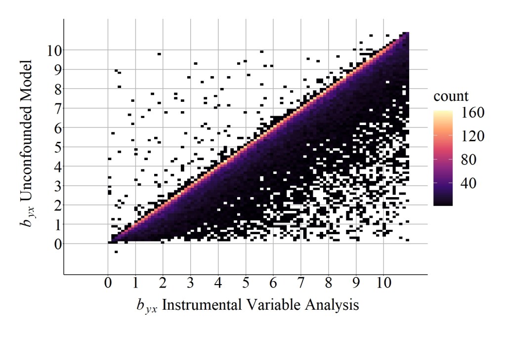
As demonstrated below, the correlation coefficient of the slope coefficient produced by the unconfounded model and the slope coefficient produced by the instrumental variable analysis was substantially weaker than the previous simulation analysis. More importantly, the median difference between the slope coefficient produced by the unconfounded model and the slope coefficient produced by the instrumental variable analysis was 0.744839750, while the mean difference was 1.185461148. These values suggest that additional bias existed when estimating the causal effects (i.e., slope coefficient) of X on Y using the instrument in Figure 2, which can be further evaluated by comparing the results in Figure 7 to the results in Figure 6.
> DF<-Example2_DATA[which(Example2_DATA$IN_byx>=0),]
>
> corr.test(DF$IN_byx,DF$M1_byx)
Call:corr.test(x = DF$IN_byx, y = DF$M1_byx)
Correlation matrix
[1] 0.71
Sample Size
[1] 49985
These are the unadjusted probability values.
  The probability values  adjusted for multiple tests are in the p.adj object.
[1] 0

 To see confidence intervals of the correlations, print with the short=FALSE option
>
> summary(DF$IN_byx-DF$M1_byx)
         Min.       1st Qu.        Median          Mean       3rd Qu.          Max.
 -6.661808399   0.355579409   0.744839750   1.185461148   1.316089008 482.423168807
>
[Figure 7]
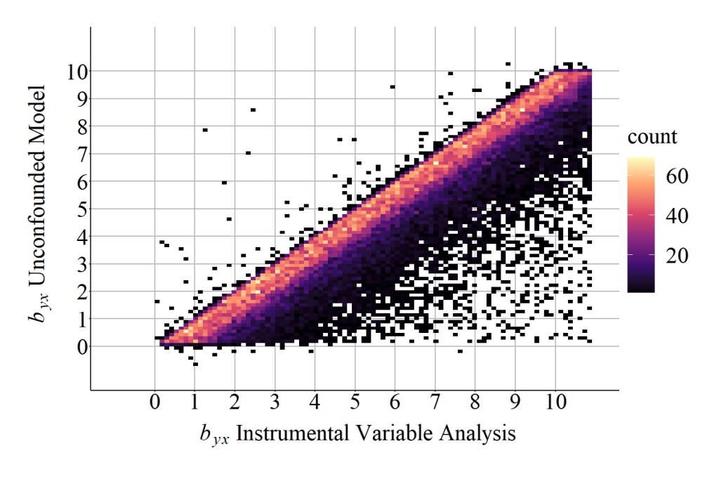
Important note: Figure 7 through Figure 10 were set on the same scale as Figure 6 to permit an observation of the pattern of findings. The linear pattern extends beyond the 10,10 coordinate in figures 7-10 and can be observed by editing the available code.
Misidentified Instrument: Variation in IN correlated with C
Using the diagram presented in Figure 3, an updated simulation analysis was conducted where variation in the instrumental variable(IN) was correlated with variation in the confounder (C).
> n<-50000
>
> set.seed(1992)
> Example3_DATA = foreach (i=1:n, .packages=c('lm.beta'), .combine=rbind) %dorng%
+   {
+     ### Value Specifications ####
+     ## Example 3 ####
+     N<-sample(150:10000, 1)
+     COR<-(rnorm(N,runif(1,-5,5),runif(1,1,30)))
+
+     IN<-runif(1,.1,10)*(rnorm(N,runif(1,-5,5),runif(1,1,30)))+runif(1,.1,10)*COR
+     Con<-runif(1,.1,10)*(rnorm(N,runif(1,-5,5),runif(1,1,30)))+runif(1,.1,10)*COR
+     X<-runif(1,.1,10)*Con+runif(1,.1,10)*IN+runif(1,.1,10)*(rnorm(N,runif(1,-5,5),runif(1,1,30)))
+     Y<-runif(1,.1,10)*Con+runif(1,.1,10)*X+runif(1,.1,10)*(rnorm(N,runif(1,-5,5),runif(1,1,30)))
+
+
+     ### Models
+     M1<-summary(lm(Y~X+Con))
+     M2<-summary(lm(Y~IN))
+     M3<-summary(lm(X~IN))
+
+     M1_byx<-coef(M1)[2, 1]
+     M2_byin<-coef(M2)[2, 1]
+     M3_bxin<-coef(M3)[2, 1]
+
+     IN_byx<-M2_byin/M3_bxin
+
+     # Data Frame ####
+
+     data.frame(i,N,M1_byx,M2_byin,M3_bxin,IN_byx)
+
+   }
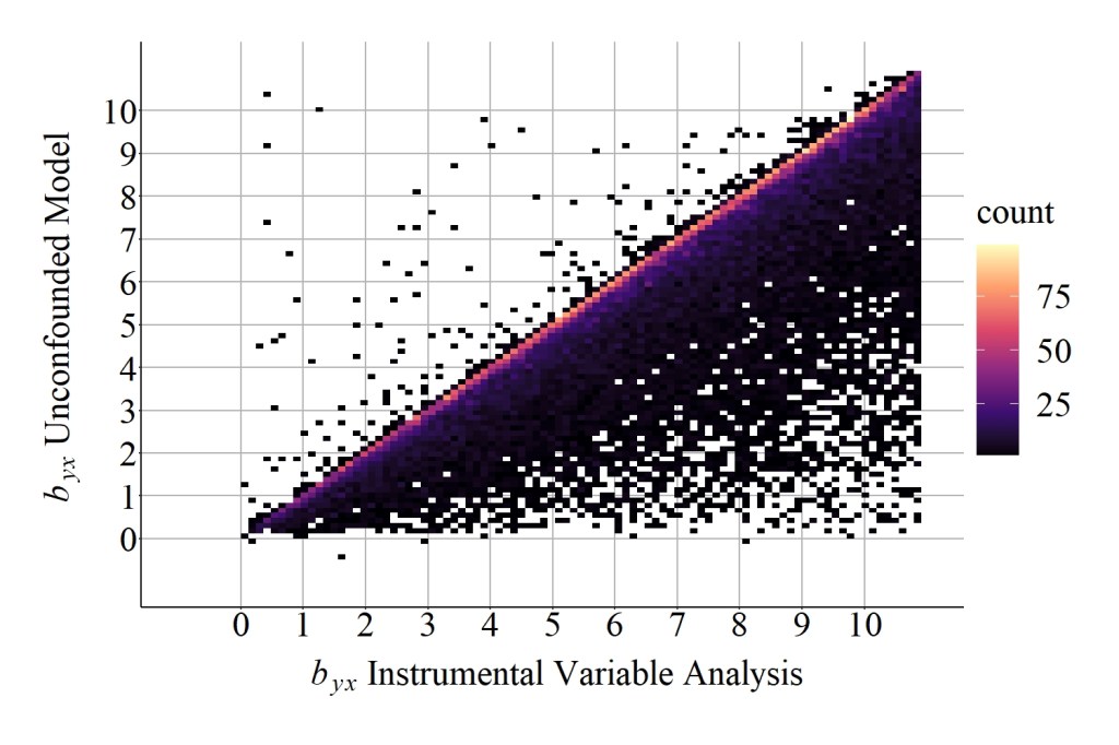
Focusing on the difference calculations, the median difference between the slope coefficient produced by the unconfounded model and the slope coefficient produced by the instrumental variable analysis was 0.1989677123 , while the mean difference was 0.3920520418. These values, again, suggest that additional bias existed when estimating the causal effects of X on Y using the instrument in Figure 3, which can be further evaluated by comparing the results in Figure 8 to the results in Figure 6. Nevertheless, the bias generated when the instrumental variable(IN) is correlated with the confounder (C) appears to be less than the bias generated when the instrumental variable(IN) causes variation in the confounder (C).
> DF<-Example3_DATA[which(Example3_DATA$IN_byx>=0),]
>
> corr.test(DF$IN_byx,DF$M1_byx)
Call:corr.test(x = DF$IN_byx, y = DF$M1_byx)
Correlation matrix
[1] 0.97
Sample Size
[1] 49993
These are the unadjusted probability values.
  The probability values  adjusted for multiple tests are in the p.adj object.
[1] 0

 To see confidence intervals of the correlations, print with the short=FALSE option
>
> summary(DF$IN_byx-DF$M1_byx)
         Min.       1st Qu.        Median          Mean       3rd Qu.          Max.
-5.2422226730  0.0532766452  0.1989677123  0.3920520418  0.4953741926 26.0382490036
[Figure 8]
Misidentified Instrument: IN causes variation in Y
Using the diagram presented in Figure 4, an updated simulation analysis was conducted where variation in the instrumental variable (IN) directly caused variation in the dependent variable (Y).
> n<-50000
>
> set.seed(1992)
> Example4_DATA = foreach (i=1:n, .packages=c('lm.beta'), .combine=rbind) %dorng%
+   {
+     ### Value Specifications ####
+     ## Example 4 ####
+     N<-sample(150:10000, 1)
+
+     IN<-(rnorm(N,runif(1,-5,5),runif(1,1,30)))
+     Con<-(rnorm(N,runif(1,-5,5),runif(1,1,30)))
+     X<-runif(1,.1,10)*Con+runif(1,.1,10)*IN+runif(1,.1,10)*(rnorm(N,runif(1,-5,5),runif(1,1,30)))
+     Y<-runif(1,.1,10)*Con+runif(1,.1,10)*X+runif(1,.1,10)*IN+runif(1,.1,10)*(rnorm(N,runif(1,-5,5),runif(1,1,30)))
+
+
+     ### Models
+     M1<-summary(lm(Y~X+Con))
+     M2<-summary(lm(Y~IN))
+     M3<-summary(lm(X~IN))
+
+     M1_byx<-coef(M1)[2, 1]
+     M2_byin<-coef(M2)[2, 1]
+     M3_bxin<-coef(M3)[2, 1]
+
+     IN_byx<-M2_byin/M3_bxin
+
+     # Data Frame ####
+
+     data.frame(i,N,M1_byx,M2_byin,M3_bxin,IN_byx)
+
+   }
As demonstrated below, the median difference between the slope coefficient produced by the unconfounded model and the slope coefficient produced by the instrumental variable analysis was 0.32667350, while the mean difference was 2.18199589. These values suggest that additional bias existed when estimating the causal effects of X on Y using the instrument in Figure 4, which can be further evaluated by comparing the results in Figure 9 to the results in Figure 6.
> DF<-Example4_DATA[which(Example4_DATA$IN_byx>=0),]
> corr.test(DF$IN_byx,DF$M1_byx)
Call:corr.test(x = DF$IN_byx, y = DF$M1_byx)
Correlation matrix
[1] 0.14
Sample Size
[1] 49713
These are the unadjusted probability values.
  The probability values  adjusted for multiple tests are in the p.adj object.
[1] 0

 To see confidence intervals of the correlations, print with the short=FALSE option
> summary(DF$IN_byx-DF$M1_byx)
         Min.       1st Qu.        Median          Mean       3rd Qu.          Max.
 -12.16465547    0.05619586    0.32667350    2.18199589    1.17082275 3179.94559972
>
[Figure 9]
Misidentified Instrument: Alternate Indirect Pathway Exists
Using the diagram presented in Figure 5, an updated simulation analysis was conducted where variation in the instrumental variable (IN) indirectly caused variation in the dependent variable (Y) through another mediator.
> n<-50000
>
> set.seed(1992)
> Example5_DATA = foreach (i=1:n, .packages=c('lm.beta'), .combine=rbind) %dorng%
+   {
+     ### Value Specifications ####
+     ## Example 5 ####
+     N<-sample(150:10000, 1)
+
+     IN<-(rnorm(N,runif(1,-5,5),runif(1,1,30)))
+     Con<-(rnorm(N,runif(1,-5,5),runif(1,1,30)))
+     M<-runif(1,.1,10)*IN+runif(1,.1,10)*(rnorm(N,runif(1,-5,5),runif(1,1,30)))
+     X<-runif(1,.1,10)*Con+runif(1,.1,10)*IN+runif(1,.1,10)*(rnorm(N,runif(1,-5,5),runif(1,1,30)))
+     Y<-runif(1,.1,10)*Con+runif(1,.1,10)*X+runif(1,.1,10)*M+runif(1,.1,10)*(rnorm(N,runif(1,-5,5),runif(1,1,30)))
+
+
+     ### Models
+     M1<-summary(lm(Y~X+Con))
+     M2<-summary(lm(Y~IN))
+     M3<-summary(lm(X~IN))
+
+     M1_byx<-coef(M1)[2, 1]
+     M2_byin<-coef(M2)[2, 1]
+     M3_bxin<-coef(M3)[2, 1]
+
+     IN_byx<-M2_byin/M3_bxin
+
+     # Data Frame ####
+
+     data.frame(i,N,M1_byx,M2_byin,M3_bxin,IN_byx)
+
+   }
As demonstrated by the results, the median difference between the slope coefficient produced by the unconfounded model and the slope coefficient produced by the instrumental variable analysis was 1.2321460, while the mean difference was 11.5971274. These values suggest that additional bias existed when estimating the causal effects of X on Y using the instrument in Figure 5, which can be further evaluated by comparing the results in Figure 10 to the results in Figure 6.
> DF<-Example5_DATA[which(Example5_DATA$IN_byx>=0),]
> corr.test(DF$IN_byx,DF$M1_byx)
Call:corr.test(x = DF$IN_byx, y = DF$M1_byx)
Correlation matrix
[1] 0.06
Sample Size
[1] 49688
These are the unadjusted probability values.
  The probability values  adjusted for multiple tests are in the p.adj object.
[1] 0

 To see confidence intervals of the correlations, print with the short=FALSE option
> summary(DF$IN_byx-DF$M1_byx)
         Min.       1st Qu.        Median          Mean       3rd Qu.          Max.
  -69.4275307     0.1881808     1.2321460    11.5971274     5.1498372 37904.7566381
>
[Figure 10]
Summary of Results, Discussion, and Conclusion
Due to concerns about the length of this entry – and the complexity of the analyses – I could not provide a comprehensive review of the results that is warranted. However, there are two important patterns that need to be highlighted to guide the conclusion. First, evident in Figure 6, a normal distribution appeared in the plot, where the highest density of bYX were the same value for both the unconfounded model and the instrumental variable analysis. This pattern is distinct from the results in figures 7-10, where it appears that the slope coefficient produced by the instrumental variable analysis was primarily upwardly biased (i.e., further from zero than the slope coefficient produced by the unconfounded model). Second, although not visually displayed, the range of differences between the bYX produced by the unconfounded model and the bYX produced by the instrumental variable analysis was substantially wider for the simulations with instrumental variables that did not satisfy the requirements of an instrument. These results, overall, demonstrate that the causal effects of X on Y can be estimated using an instrumental variable analysis when employing a construct that satisfies the requirements of an instrument. Nevertheless, when the construct does not satisfy the requirements of an instrument, the estimated effects of X on Y produced by an instrumental variable analysis is commonly upwardly biased – further from zero than the true causal effects.
Typically, I do not introduce philosophical debates into this series, but I do believe that it is required when discussing sources of bias in an instrumental variable analysis. If you have ever participated in a research methods or statistics course, one of the first things you are taught is that you can not rule out unobserved confounders in non-experimental research. This directly translates to, you can not rule out unobserved causes and causal pathways. Now, take a glance at figures 1-5 again and think of a scenario where you can definitively identify an instrument. That is, it can not cause or be correlated with variation in the confounder, it can not directly cause variation in the dependent variable, and it can not indirectly cause variation in the dependent variable through an alternative path. Can you truly think of or find any? So I ask, knowing that violating the requirements of an instrument can reduce your ability to observe the causal effects between constructs, are the benefits of an instrumental variable analysis diminished by the inability to intrinsically define any construct as a true instrument? Do the benefits of the technique outweigh the shortcomings?
p.s. I have no bearing on your implementation of instrumental variable analysis – as long as you think it is the best approach for the research at hand please do not let me dissuade you. It, however, is always good practice to note the assumptions and limitations of the technique.
License: Creative Commons Attribution 4.0 International (CC By 4.0)
