You might have the thought of: I know the constructs that can confound, mediate, or moderate the association I am interested in, and I am surely not going to include a collider as a covariate in my regression model! You also, like a great student of causal inference, have embraced the process of creating a directed acyclic graph (DAG) to guide the selection of your covariates. I, however, have to ask, did you consider if any of those covariates are descendants of confounders, mediators, moderators, or colliders? If not, let’s spend some time talking about the importance of descendants and, if so, you can probably skip over this entry … just kidding. Descendants, just like their ancestors (terms described below), under some conditions can be used to reduce bias, while under other conditions, the introduction of a descendant can increase the bias in our statistical estimates. In this entry we will review how the inclusion of descendants in our statistical models can increase or decrease – depending upon the ancestor – the bias in the estimates corresponding with the association of interest.
Descendants
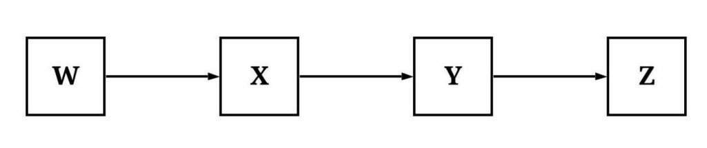
Within most scientific disciplines, we use the terms independent variable and dependent variable – or exogenous, lagged endogenous, and endogenous variables – to describe the construct we believe is causing variation and the construct that has variation being caused. These terms, although really designed to ease model specification, present problems when describing causal pathways in structural systems. That is, it is confusing to use terms like lagged endogenous variables or dependent variables to describe all of the causes and mechanisms being caused when discussing complicated structural systems. As such, the kinship terms of parent, child, ancestor, and descendent have been adopted to ease the description of structural systems. Briefly, a parent is a construct that causes variation in a child (a direct descendant). If the parent is also a child (i.e., variation caused by a 1st generation), the indirect cause of the variation to the 2nd generation is an ancestor, while the child in the 2nd generation is a descendant of both the parent and the ancestor. I know it can be confusing, so let’s apply these kinship terms to the causal pathway illustrated below.
If we assume the pathways below represent causal relationships, the figure demonstrates that variation in W causes variation in X, which causes variation in Y, which in turn causes variation in Z. Using the kinship terms, W is a parent to X and an ancestor to Y and Z because X is the parent of Y and Y is the parent of Z. Alternatively, Y and Z are descendants of W because X is a child to W, Y is a child to X, and Z is a child to Y. While it might take some time to get used to the nomenclature, out of my own preference I typically only use the terms ancestors and descendants because in practice we can not easily identify a child or a parent. As such, X, Y, and Z are descendants of W because variation in these constructs is causally influenced by variation in W.
The Importance of Descendants
The best way to understand the importance of descendants when specifying a statistical model is through a series of simulated illustrations. Nevertheless, before we work through our illustrations, let’s briefly define the variation in a descendant. The variation in a descendant is comprised of two components: (1) shared variation with the ancestors and (2) variation unique to the descendant. The further a descendant is from an ancestor (in the causal pathway), the less variation a descendant shares with that ancestor. The amount of variation shared is proportional to the variation shared by ancestor-descendant pairs and the number of mediating constructs along the causal pathway. Given the shared variation, adjusting for a descendant in a statistical model can indirectly adjust for the variation associated with the ancestors. By adjusting for the descendants of key constructs within a statistical model, and indirectly adjusting for the variation in the ancestor, we can reduce or increase the bias in the estimates corresponding to the association of interest. Let’s begin our illustrations by focusing on the descendants of confounders.
Descendants of Confounders
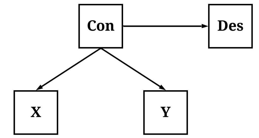
When referencing a descendant of a confounder, we are discussing a mechanism causally influenced by the variation in the confounder, but not causally associated with the association of interest. This is demonstrated in the figure below, where Con (short for confounder) causally influences both X and Y (i.e., X and Y are descendants of Con) but the variation in X does not causally influence the variation in Y. Under these conditions, a statistical model will suggest that X causes variation in Y unless the model is conditioned upon Con. Importantly, Des is also causally influenced by Con, creating identical conditions where the lack of causal influence between X and Des and Y and Des will not be revealed unless the statistical model is conditioned upon Con. Although these identical conditions exist, the focus of the example below will be the causal association between X and Y.
To simulate our structural system – the causal pathways within the figure –, we will simulate Con first and then simulate the descendants (X, Y, and Des). Evident in the syntax below, we simulated a dataset of 1000 cases, where all of the measures were specified to be normally distributed with a mean of zero. Moreover, variation in X, Y, and Des were specified to be causally influenced by variation in Con, but the amount of variation in DES causally influenced by Con was substantially larger than the amount of variation in X and Y causally influenced by Con. This specification makes Des an extremely good approximation of Con. Moreover, using the syntax below we can ensure that the variation in X has no causal influence on the variation in Y.
> ## Example 1 ####
> n<-1000
>
> set.seed(1992)
> Con<-rnorm(n,0,10)
> X<-2*Con+.50*rnorm(n,0,10)
> Y<-2*Con+.00*X+.50*rnorm(n,0,10)
> Des<-20*Con+1*rnorm(n,0,10)
Now that we have our data, let’s estimate three models: (1) the bivariate association between X and Y, (2) the association between X and Y adjusting for Con, and (3) the association between X and Y adjusting for Des. Focusing on the first model, when Y is regressed on X without adjusting for Con the statistical estimates suggest that variation in X causally influences variation in Y. The slope coefficient of .930 suggests that a 1 point change in X is associated with a .930 change in Y.
> summary(lm(Y~X))

Call:
lm(formula = Y ~ X)

Residuals:
          Min            1Q        Median            3Q           Max
-23.626283367  -4.734664574  -0.164041357   4.520330368  25.280209778

Coefficients:
                 Estimate    Std. Error  t value             Pr(>|t|)
(Intercept) -0.3675314299  0.2235938024 -1.64375              0.10054
X            0.9295740269  0.0111141701 83.63864 < 0.0000000000000002 ***
---
Signif. codes:  0 ‘***’ 0.001 ‘**’ 0.01 ‘*’ 0.05 ‘.’ 0.1 ‘ ’ 1

Residual standard error: 7.0705672 on 998 degrees of freedom
Multiple R-squared:  0.87514733,	Adjusted R-squared:  0.875022227
F-statistic: 6995.42136 on 1 and 998 DF,  p-value: < 0.0000000000000002220446

> lm.beta(lm(Y~X))

Call:
lm(formula = Y ~ X)

Standardized Coefficients::
   (Intercept)              X
0.000000000000 0.935493094548

>
After adjusting for the variation in Con, however, the findings suggest that variation in X does not causally influence variation in Y. The slope coefficient of -.043 should not come as a surprise, given our previous discussions about confounder bias (Entry 7). The estimates presented below represent the unconfounded association and is a substantial departure from the estimates representing the confounded association (the preceding model).
> summary(lm(Y~X+Con))

Call:
lm(formula = Y ~ X + Con)

Residuals:
          Min            1Q        Median            3Q           Max
-19.455680213  -3.487189970  -0.301747267   3.282097622  16.863658189

Coefficients:
                 Estimate    Std. Error  t value             Pr(>|t|)
(Intercept) -0.0980793972  0.1598106304 -0.61372              0.53954
X           -0.0432708159  0.0323468275 -1.33771              0.18129
Con          2.0710151227  0.0667582688 31.02260 < 0.0000000000000002 ***
---
Signif. codes:  0 ‘***’ 0.001 ‘**’ 0.01 ‘*’ 0.05 ‘.’ 0.1 ‘ ’ 1

Residual standard error: 5.04612237 on 997 degrees of freedom
Multiple R-squared:  0.936471369,	Adjusted R-squared:  0.936343929
F-statistic: 7348.35566 on 2 and 997 DF,  p-value: < 0.0000000000000002220446

> lm.beta(lm(Y~X+Con))

Call:
lm(formula = Y ~ X + Con)

Standardized Coefficients::
     (Intercept)                X              Con
 0.0000000000000 -0.0435463430992  1.0098723974868
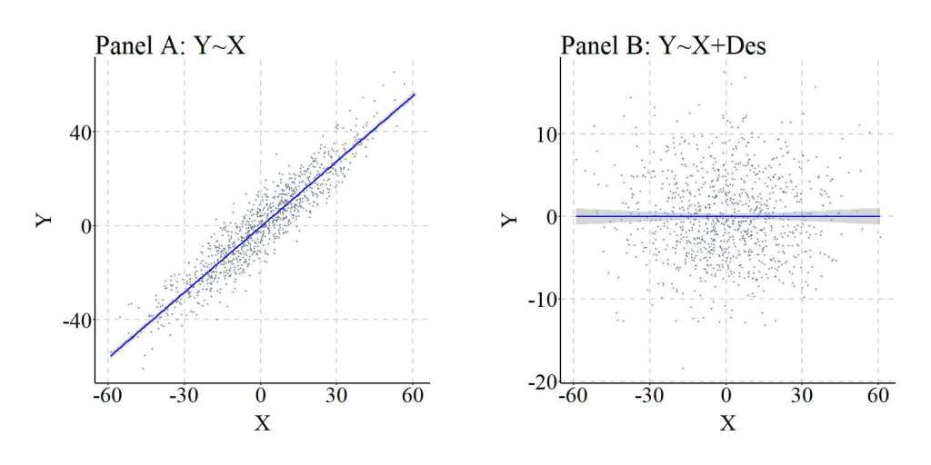
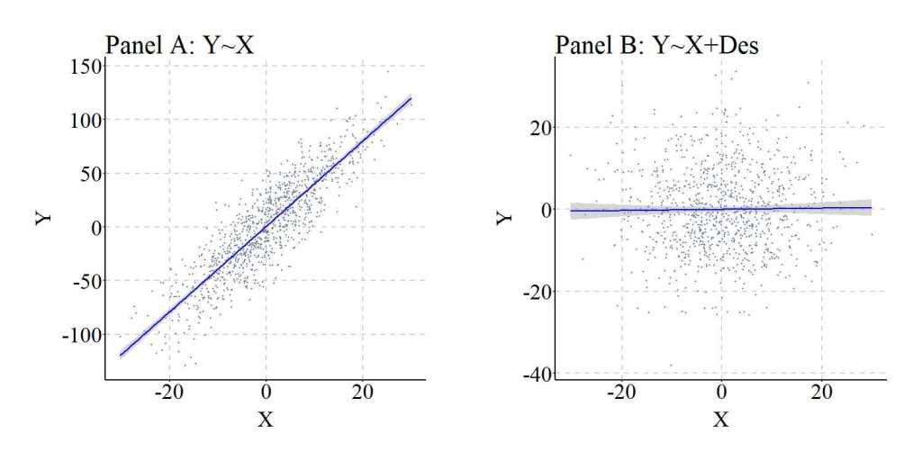
Just for a second, though, let’s imagine that we can not observe or capture variation in Con. As such, we are left searching for an approximation and stumble upon Des, which we then plug into our model. Oh my, the slope coefficient and standardized slope coefficient for the association between X and Y are almost identical to the estimates produced when we adjusted for Con in our statistical model. Although differences do exist – because the variation in Des is not identical to the variation in Con –, the slope coefficient produced when adjusting for the variation in Des is substantially closer to the unconfounded model than the confounded model. Importantly, the findings suggest that variation in Des causally influences variation in Y – which we know is false –, requiring the development of a Directed Acyclic Graph (DAG) to accurately interpret the estimated associations.
> summary(lm(Y~X+Des))

Call:
lm(formula = Y ~ X + Des)

Residuals:
         Min           1Q       Median           3Q          Max
-18.47467968  -3.63240155  -0.36160646   3.37157472  17.52413891

Coefficients:
                  Estimate     Std. Error  t value             Pr(>|t|)
(Intercept) -0.14713163065  0.16408631510 -0.89667              0.37011
X            0.00625869336  0.03252152764  0.19245              0.84743
Des          0.09837471729  0.00335450446 29.32615 < 0.0000000000000002 ***
---
Signif. codes:  0 ‘***’ 0.001 ‘**’ 0.01 ‘*’ 0.05 ‘.’ 0.1 ‘ ’ 1

Residual standard error: 5.18335365 on 997 degrees of freedom
Multiple R-squared:  0.932969011,	Adjusted R-squared:  0.932834546
F-statistic: 6938.35882 on 2 and 997 DF,  p-value: < 0.0000000000000002220446

> lm.beta(lm(Y~X+Des))

Call:
lm(formula = Y ~ X + Des)

Standardized Coefficients::
     (Intercept)                X              Des
0.00000000000000 0.00629854562082 0.95980424619948

>
The differences between the confounded model and the model adjusting for Des are further illustrated in the figure below.
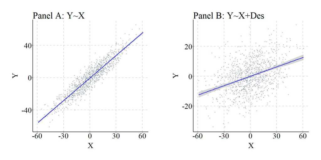
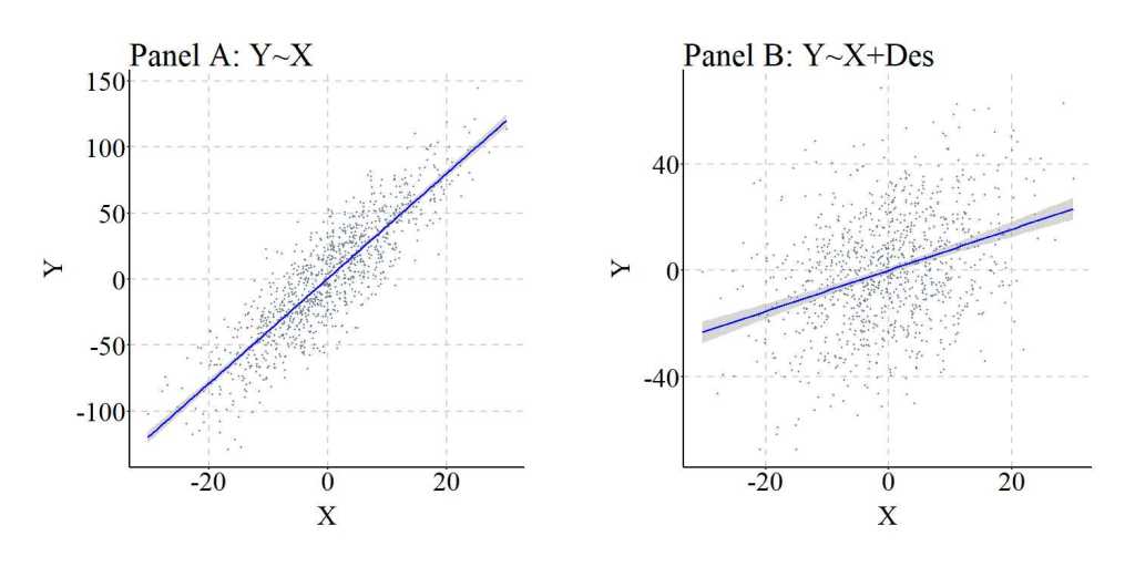
As a replication, we can simulate the data again but weakened the causal influence of Con on Des, reducing the ability of Des to serve as an approximation of Con. Evident by the findings of the replication, the amount of variation shared between Con and Des directly influences the ability of Des to adjust for confounder bias when estimating the causal effects of X on Y. In particular, while the estimated association between X and Y is attenuated, under these circumstances adjusting for the variation in Des can not produce estimates representative of the specified causal association.
> ## Example 2 ####
> n<-1000
>
> set.seed(1992)
> Con<-rnorm(n,0,10)
> X<-2*Con+.50*rnorm(n,0,10)
> Y<-2*Con+.00*X+.50*rnorm(n,0,10)
> Des<-2*Con+1*rnorm(n,0,10)
>
> summary(lm(Y~X))

Call:
lm(formula = Y ~ X)

Residuals:
          Min            1Q        Median            3Q           Max
-23.626283367  -4.734664574  -0.164041357   4.520330368  25.280209778

Coefficients:
                 Estimate    Std. Error  t value             Pr(>|t|)
(Intercept) -0.3675314299  0.2235938024 -1.64375              0.10054
X            0.9295740269  0.0111141701 83.63864 < 0.0000000000000002 ***
---
Signif. codes:  0 ‘***’ 0.001 ‘**’ 0.01 ‘*’ 0.05 ‘.’ 0.1 ‘ ’ 1

Residual standard error: 7.0705672 on 998 degrees of freedom
Multiple R-squared:  0.87514733,	Adjusted R-squared:  0.875022227
F-statistic: 6995.42136 on 1 and 998 DF,  p-value: < 0.0000000000000002220446

> lm.beta(lm(Y~X))

Call:
lm(formula = Y ~ X)

Standardized Coefficients::
   (Intercept)              X
0.000000000000 0.935493094548

>
> summary(lm(Y~X+Des))

Call:
lm(formula = Y ~ X + Des)

Residuals:
          Min            1Q        Median            3Q           Max
-21.281840236  -4.740428993  -0.087244974   4.542584785  24.360961565

Coefficients:
                 Estimate    Std. Error  t value             Pr(>|t|)
(Intercept) -0.3845427252  0.2153325869 -1.78581             0.074434 .
X            0.7736553380  0.0205372816 37.67078 < 0.0000000000000002 ***
Des          0.1675961926  0.0188405306  8.89551 < 0.0000000000000002 ***
---
Signif. codes:  0 ‘***’ 0.001 ‘**’ 0.01 ‘*’ 0.05 ‘.’ 0.1 ‘ ’ 1

Residual standard error: 6.80905941 on 997 degrees of freedom
Multiple R-squared:  0.884328015,	Adjusted R-squared:  0.884095975
F-statistic:  3811.1001 on 2 and 997 DF,  p-value: < 0.0000000000000002220446

> lm.beta(lm(Y~X+Des))

Call:
lm(formula = Y ~ X + Des)

Standardized Coefficients::
   (Intercept)              X            Des
0.000000000000 0.778581592531 0.183852941585
Descendants of Colliders
Similar to a descendant of a confounder, a descendant of a collider refers to a construct causally influenced by the variation in a collider unrelated to the association of interest. As demonstrated below, variation in Col (short for collider) causally influences variation in Des, but variation in Col is now causally influenced by variation in both X and Y.
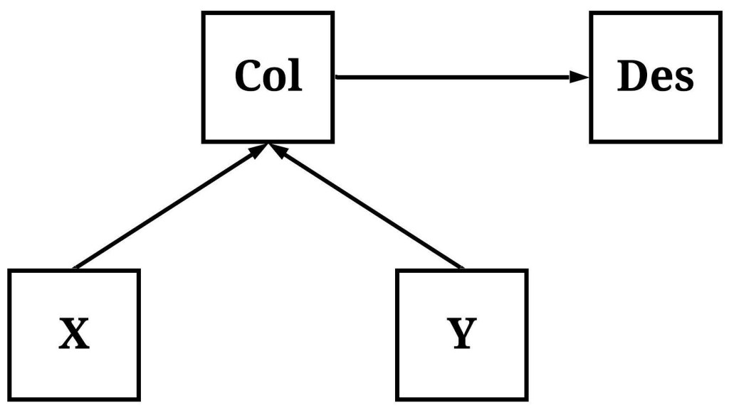
To simulate data following the structural system presented above, we reverse the order of the simulation and specify the distribution of scores on X and Y first. After simulating X and Y, we can specify that Col is causally influenced by the variation in X and Y, and causally influences the variation in Des. The specification of the association between Col and Des below generates a condition where Des is almost a perfect approximation of Col.
## Example 1 ####
n<-1000

set.seed(1992)
X<-rnorm(n,0,10)
Y<-rnorm(n,0,10)
Col<-2*X+2*Y+rnorm(n,0,10)
Des<-20*Col+1*rnorm(n,0,10)
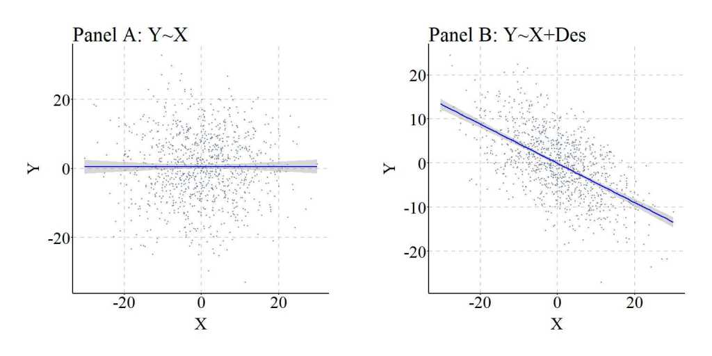
Following the process detailed above, three linear regression models were estimated where: (1) Y was regressed on X, (2) Y was regressed on X and Col, and (3) Y was regressed on X and Des. As presented below, the estimates produced in the bivariate regression model present evidence suggesting that X does not causally influence Y, while the regression model adjusting for Col suggests that X does causally influence Y. The bias in the estimates, as expected given Entry 8 in the series, corresponds with the introduction of the collider into a regression model. Importantly, Model 3 produced estimates almost identical to the model adjusting for the variation in Col, suggesting that the variation in Des can generate collider bias if Des is a descendant of a collider. The bias generated by adjusting for Des – a descendant of a collider – is further demonstrated in a figure below.
Bivariate Model
> summary(lm(Y~X))

Call:
lm(formula = Y ~ X)

Residuals:
         Min           1Q       Median           3Q          Max
-33.39823634  -6.39223268  -0.12454071   6.77441730  32.32615833

Coefficients:
                Estimate   Std. Error t value Pr(>|t|)
(Intercept) 0.5328217473 0.3123247274 1.70599 0.088322 .
X           0.0016311375 0.0320395916 0.05091 0.959407
---
Signif. codes:  0 ‘***’ 0.001 ‘**’ 0.01 ‘*’ 0.05 ‘.’ 0.1 ‘ ’ 1

Residual standard error: 9.87622125 on 998 degrees of freedom
Multiple R-squared:  2.59702143e-06,	Adjusted R-squared:  -0.000999404384
F-statistic: 0.00259183411 on 1 and 998 DF,  p-value: 0.959407377

> lm.beta(lm(Y~X))

Call:
lm(formula = Y ~ X)

Standardized Coefficients::
     (Intercept)                X
0.00000000000000 0.00161152766817
Model Adjusting for the Collider
> summary(lm(Y~X+Col))

Call:
lm(formula = Y ~ X + Col)

Residuals:
          Min            1Q        Median            3Q           Max
-13.543830672  -2.946857580   0.158945553   2.951317200  16.910867430

Coefficients:
                  Estimate     Std. Error   t value             Pr(>|t|)
(Intercept)  0.19287028087  0.14470345773   1.33287              0.18288
X           -0.79043929094  0.01978553859 -39.95036 < 0.0000000000000002 ***
Col          0.40163018863  0.00663937684  60.49215 < 0.0000000000000002 ***
---
Signif. codes:  0 ‘***’ 0.001 ‘**’ 0.01 ‘*’ 0.05 ‘.’ 0.1 ‘ ’ 1

Residual standard error: 4.57230915 on 997 degrees of freedom
Multiple R-squared:  0.785882067,	Adjusted R-squared:  0.785452543
F-statistic: 1829.65624 on 2 and 997 DF,  p-value: < 0.0000000000000002220446

> lm.beta(lm(Y~X+Col))

Call:
lm(formula = Y ~ X + Col)

Standardized Coefficients::
    (Intercept)               X             Col
 0.000000000000 -0.780936486139  1.182480809249

>
Model Adjusting for the Descendant of the Collider
> summary(lm(Y~X+Des))

Call:
lm(formula = Y ~ X + Des)

Residuals:
          Min            1Q        Median            3Q           Max
-13.509839731  -2.973642429   0.149793824   2.944323483  17.154745121

Coefficients:
                   Estimate      Std. Error   t value             Pr(>|t|)
(Intercept)  0.185652395314  0.144691697215   1.28309              0.19976
X           -0.790051816042  0.019778785457 -39.94440 < 0.0000000000000002 ***
Des          0.020081846598  0.000331926437  60.50090 < 0.0000000000000002 ***
---
Signif. codes:  0 ‘***’ 0.001 ‘**’ 0.01 ‘*’ 0.05 ‘.’ 0.1 ‘ ’ 1

Residual standard error: 4.57178981 on 997 degrees of freedom
Multiple R-squared:  0.785930705,	Adjusted R-squared:  0.785501278
F-statistic: 1830.18521 on 2 and 997 DF,  p-value: < 0.0000000000000002220446

> lm.beta(lm(Y~X+Des))

Call:
lm(formula = Y ~ X + Des)

Standardized Coefficients::
    (Intercept)               X             Des
 0.000000000000 -0.780553669535  1.182248072119

>
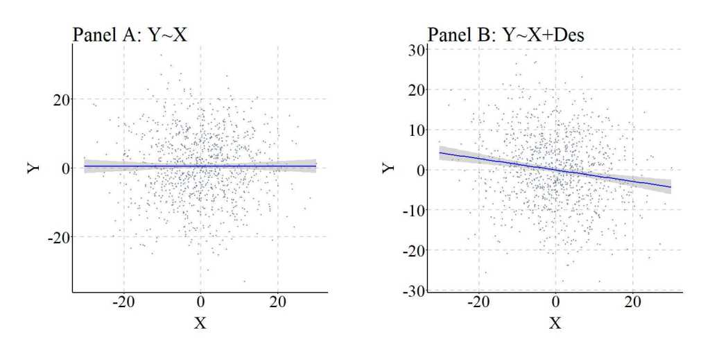
Nevertheless, similar to the previous example this is an extreme case where almost all of the variation in Des is caused by Col. As such, we can replicate the previous simulation but weaken the causal influence of Col on Des. The findings and figures are presented below and further demonstrate that adjusting for the descendant of a collider can introduce collider bias into the estimates corresponding with the association of interest.
> ## Example 2 ####
> n<-1000
>
> set.seed(1992)
> X<-rnorm(n,0,10)
> Y<-rnorm(n,0,10)
> Col<-2*X+2*Y+rnorm(n,0,10)
> Des<-.25*Col+1*rnorm(n,0,10)
>
>
> summary(lm(Y~X))

Call:
lm(formula = Y ~ X)

Residuals:
         Min           1Q       Median           3Q          Max
-33.39823634  -6.39223268  -0.12454071   6.77441730  32.32615833

Coefficients:
                Estimate   Std. Error t value Pr(>|t|)
(Intercept) 0.5328217473 0.3123247274 1.70599 0.088322 .
X           0.0016311375 0.0320395916 0.05091 0.959407
---
Signif. codes:  0 ‘***’ 0.001 ‘**’ 0.01 ‘*’ 0.05 ‘.’ 0.1 ‘ ’ 1

Residual standard error: 9.87622125 on 998 degrees of freedom
Multiple R-squared:  2.59702143e-06,	Adjusted R-squared:  -0.000999404384
F-statistic: 0.00259183411 on 1 and 998 DF,  p-value: 0.959407377

> lm.beta(lm(Y~X))

Call:
lm(formula = Y ~ X)

Standardized Coefficients::
     (Intercept)                X
0.00000000000000 0.00161152766817

>
> summary(lm(Y~X+Des))

Call:
lm(formula = Y ~ X + Des)

Residuals:
         Min           1Q       Median           3Q          Max
-28.76071481  -5.82984012   0.04863643   6.06431850  27.29574583

Coefficients:
                 Estimate    Std. Error  t value               Pr(>|t|)
(Intercept)  0.3333244798  0.2847473164  1.17060                0.24204
X           -0.1637272299  0.0313627762 -5.22043           0.0000002172 ***
Des          0.3495374707  0.0243220826 14.37120 < 0.000000000000000222 ***
---
Signif. codes:  0 ‘***’ 0.001 ‘**’ 0.01 ‘*’ 0.05 ‘.’ 0.1 ‘ ’ 1

Residual standard error: 8.99347184 on 997 degrees of freedom
Multiple R-squared:  0.171606606,	Adjusted R-squared:  0.169944834
F-statistic: 103.267233 on 2 and 997 DF,  p-value: < 0.0000000000000002220446

> lm.beta(lm(Y~X+Des))

Call:
lm(formula = Y ~ X + Des)

Standardized Coefficients::
    (Intercept)               X             Des
 0.000000000000 -0.161758871352  0.445302028509

>
Descendants of Mediators
Descendants of mediators are constructs causally influenced by the mechanism mediating the association of interest. Take for example the figure below, where the variation in X causally influences the variation in Me which, in turn, causally influences the variation in Des and the variation in Y. As the trend as begun to appear, adjusting for Des – under these conditions – will function similarly to adjusting for Me, reducing our ability to observe the total causal effects of X on Y and only permitting the observation of the direct causal effects.
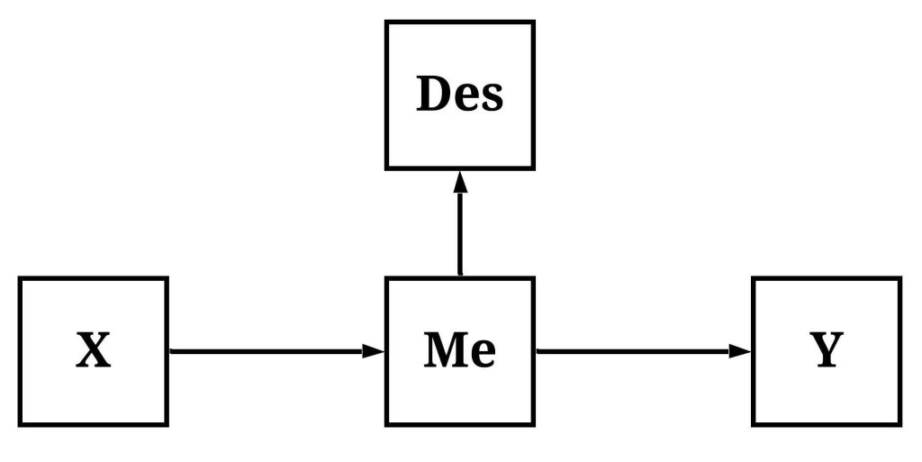
To simulate data following the structural specification outlined in the figure, we must first simulate variation in X. After which, we can specify that X causally influences variation in M, which can be specified to causally influence variation in Y and variation in Des. Following a consistent pattern, the specification below is designed to make the variation in Des almost identical to the variation in M.
## Example 1 ####
n<-1000

set.seed(1992)
X<-rnorm(n,0,10)
M<-2*X+rnorm(n,0,10)
Y<-2*M+rnorm(n,0,10)
Des<-20*M+1*rnorm(n,0,10)
After simulating the data, we can again estimate our three regression models: (1) Y regressed on X, (2) Y regressed on X and M, and (3) Y regressed on X and Des. As a reminder, the first model will provide estimates representative of the total causal effects of X on Y, while the second and third models will produce estimates representative of only the direct causal effects of X on Y. If we are interested in the total causal effects of X on Y, adjusting for the variation in M or the variation in Des will provide estimates not representative of the desired causal effects.
The effects of adjusting for the mediator and the descendant of a mediator is demonstrated below, where the bivariate association highlights that variation in X does causally influence variation in Y, but the models adjusting for M or Des suggest that X does not causally influence variation in Y (because X does not directly cause variation in Y). Importantly, the association between M and Y is substantially larger than the association between Des and Y, suggesting that the variation shared between Des and M might not perfectly emulate the variation shared between M and Y. The effects of adjusting for Des, under these conditions, is further demonstrated in the figure below.
Bivariate Model
> summary(lm(Y~X))

Call:
lm(formula = Y ~ X)

Residuals:
         Min           1Q       Median           3Q          Max
-69.81609609 -14.16806065   0.07581825  15.30999351  63.58971146

Coefficients:
                Estimate   Std. Error  t value             Pr(>|t|)
(Intercept) 0.8464290685 0.6893798040  1.22781              0.21981
X           3.9721386760 0.0707194962 56.16752 < 0.0000000000000002 ***
---
Signif. codes:  0 ‘***’ 0.001 ‘**’ 0.01 ‘*’ 0.05 ‘.’ 0.1 ‘ ’ 1

Residual standard error: 21.7993225 on 998 degrees of freedom
Multiple R-squared:  0.759679651,	Adjusted R-squared:  0.759438849
F-statistic: 3154.79024 on 1 and 998 DF,  p-value: < 0.0000000000000002220446

> lm.beta(lm(Y~X))

Call:
lm(formula = Y ~ X)

Standardized Coefficients::
   (Intercept)              X
0.000000000000 0.871596036565

> 0.00000000000000 0.00161152766817
Model Adjusting for the Mediator
> summary(lm(Y~X+M))

Call:
lm(formula = Y ~ X + M)

Residuals:
         Min           1Q       Median           3Q          Max
-38.91136043  -6.97437994  -0.60349453   6.56419524  33.72731638

Coefficients:
                 Estimate    Std. Error  t value             Pr(>|t|)
(Intercept) -0.1961587943  0.3196212609 -0.61372              0.53954
X            0.0554886135  0.0725536497  0.76479              0.44458
M            1.9567291841  0.0323468275 60.49215 < 0.0000000000000002 ***
---
Signif. codes:  0 ‘***’ 0.001 ‘**’ 0.01 ‘*’ 0.05 ‘.’ 0.1 ‘ ’ 1

Residual standard error: 10.0922447 on 997 degrees of freedom
Multiple R-squared:  0.94854297,	Adjusted R-squared:  0.948439746
F-statistic: 9189.19477 on 2 and 997 DF,  p-value: < 0.0000000000000002220446

> lm.beta(lm(Y~X+M))

Call:
lm(formula = Y ~ X + M)

Standardized Coefficients::
    (Intercept)               X               M
0.0000000000000 0.0121757218428 0.9630506718006

>
Model Adjusting for the Descendant of the Mediator
> summary(lm(Y~X+Des))

Call:
lm(formula = Y ~ X + Des)

Residuals:
         Min           1Q       Median           3Q          Max
-37.68591523  -6.95585465  -0.62557652   6.60579653  33.72367847

Coefficients:
                  Estimate     Std. Error  t value             Pr(>|t|)
(Intercept) -0.22738900718  0.32216328928 -0.70582              0.48047
X            0.07163169784  0.07300878543  0.98114              0.32676
Des          0.09748180748  0.00162764264 59.89141 < 0.0000000000000002 ***
---
Signif. codes:  0 ‘***’ 0.001 ‘**’ 0.01 ‘*’ 0.05 ‘.’ 0.1 ‘ ’ 1

Residual standard error: 10.171544 on 997 degrees of freedom
Multiple R-squared:  0.947731151,	Adjusted R-squared:  0.947626299
F-statistic:  9038.7294 on 2 and 997 DF,  p-value: < 0.0000000000000002220446

> lm.beta(lm(Y~X+Des))

Call:
lm(formula = Y ~ X + Des)

Standardized Coefficients::
   (Intercept)              X            Des
0.000000000000 0.015717956753 0.959467971278

>
Again, we can replicate this simulation while reducing the causal effects of M on Des. The findings of the replication are presented below.
> ## Example 2 ####
> n<-1000
>
>
> set.seed(1992)
> X<-rnorm(n,0,10)
> M<-2*X+rnorm(n,0,10)
> Y<-2*M+rnorm(n,0,10)
> Des<-1*M+1*rnorm(n,0,10)
>
>
> summary(lm(Y~X))

Call:
lm(formula = Y ~ X)

Residuals:
         Min           1Q       Median           3Q          Max
-69.81609609 -14.16806065   0.07581825  15.30999351  63.58971146

Coefficients:
                Estimate   Std. Error  t value             Pr(>|t|)
(Intercept) 0.8464290685 0.6893798040  1.22781              0.21981
X           3.9721386760 0.0707194962 56.16752 < 0.0000000000000002 ***
---
Signif. codes:  0 ‘***’ 0.001 ‘**’ 0.01 ‘*’ 0.05 ‘.’ 0.1 ‘ ’ 1

Residual standard error: 21.7993225 on 998 degrees of freedom
Multiple R-squared:  0.759679651,	Adjusted R-squared:  0.759438849
F-statistic: 3154.79024 on 1 and 998 DF,  p-value: < 0.0000000000000002220446

> lm.beta(lm(Y~X))

Call:
lm(formula = Y ~ X)

Standardized Coefficients::
   (Intercept)              X
0.000000000000 0.871596036565

>
> summary(lm(Y~X+Des))

Call:
lm(formula = Y ~ X + Des)

Residuals:
         Min           1Q       Median           3Q          Max
-55.60249098 -11.80836898  -0.33076703  12.56735897  54.59397296

Coefficients:
                Estimate   Std. Error  t value             Pr(>|t|)
(Intercept) 0.0330722183 0.5522890161  0.05988              0.95226
X           2.1650996171 0.0948040714 22.83762 < 0.0000000000000002 ***
Des         0.9118749831 0.0383986518 23.74758 < 0.0000000000000002 ***
---
Signif. codes:  0 ‘***’ 0.001 ‘**’ 0.01 ‘*’ 0.05 ‘.’ 0.1 ‘ ’ 1

Residual standard error: 17.4306717 on 997 degrees of freedom
Multiple R-squared:  0.846503875,	Adjusted R-squared:  0.846195959
F-statistic: 2749.13898 on 2 and 997 DF,  p-value: < 0.0000000000000002220446

> lm.beta(lm(Y~X+Des))

Call:
lm(formula = Y ~ X + Des)

Standardized Coefficients::
   (Intercept)              X            Des
0.000000000000 0.475082165797 0.494011612561

>
Descendants of Moderators
Consistent with the previous discussions, in the current context a descendant of a moderator refers to a construct causally influenced by the variation in a mechanism moderating the association of interest. This, as illustrated below, means that variation in X does causally influence variation in Y, but the magnitude of the association changes at different levels of Mo. Moreover, the variation in Mo causally influences the variation in Des.

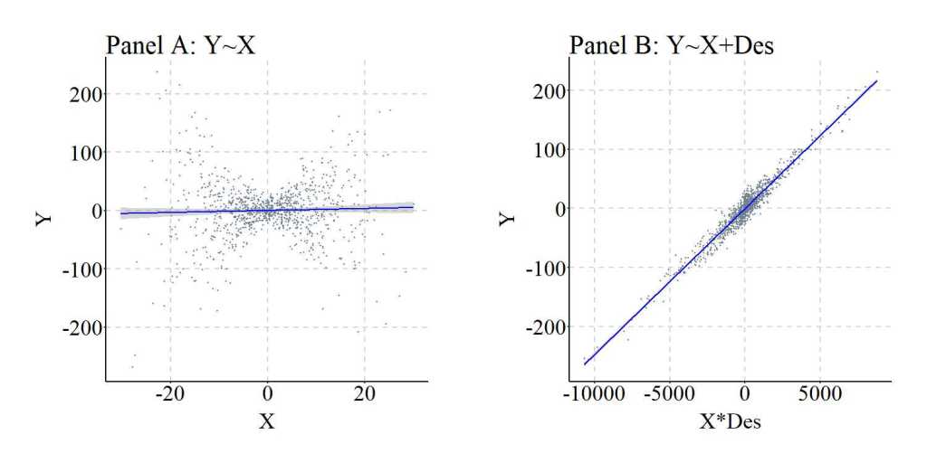
To simulate the data, X and M (sorry the syntax uses M for Mo) are specified as continuous normally distributed variables, while Y is specified to be normally distributed and causally influenced by only the interaction between X and M. This is evident by the specification of X*M. Des was specified to be causally influenced by M. Three regression models were specified to examine the effects of including an interaction between X and Des in the model: (1) Y regressed on X, (2) Y regressed on X, M, and an interaction between X and M, and (3) Y regressed on X, Des, and an interaction between X and Des. Evident by the results, Des – when variation in Des is causally influenced by variation in M – functions similarly to M in that including an interaction between Des and X demonstrates that X does causally influence Y. The magnitude of the causal effects of X on Y does vary by M. It is important, however, to note that the magnitude of the interaction effects is substantially diminished when comparing the interaction estimates corresponding to X*M to the interaction estimates corresponding to X*Des. This attenuation is likely the product of the residual variation in Des (i.e., the variation unique to Des).
Bivariate Model
> summary(lm(Y~X))

Call:
lm(formula = Y ~ X)

Residuals:
          Min            1Q        Median            3Q           Max
-263.41802778  -20.08017285    0.26256427   21.08051513  242.35063198

Coefficients:
                Estimate   Std. Error  t value Pr(>|t|)
(Intercept) -0.147056842  1.561068597 -0.09420  0.92497
X            0.170546456  0.160141020  1.06498  0.28714

Residual standard error: 49.363555 on 998 degrees of freedom
Multiple R-squared:  0.00113515824,	Adjusted R-squared:  0.000134291665
F-statistic: 1.13417539 on 1 and 998 DF,  p-value: 0.287144056

> lm.beta(lm(Y~X))

Call:
lm(formula = Y ~ X)

Standardized Coefficients::
    (Intercept)               X
0.0000000000000 0.0336921094564
Model Adjusting for the Moderator
> summary(lm(Y~X+M+X*M))

Call:
lm(formula = Y ~ X + M + X * M)

Residuals:
         Min           1Q       Median           3Q          Max
-38.91513976  -6.97454924  -0.60176279   6.56371310  33.72800861

Coefficients:
                  Estimate     Std. Error   t value             Pr(>|t|)
(Intercept) -0.19611564507  0.31978882353  -0.61327              0.53984
X           -0.03102597597  0.03278451867  -0.94636              0.34419
M           -0.04333370793  0.03251416397  -1.33276              0.18291
X:M          0.49993320824  0.00332520586 150.34654 < 0.0000000000000002 ***
---
Signif. codes:  0 ‘***’ 0.001 ‘**’ 0.01 ‘*’ 0.05 ‘.’ 0.1 ‘ ’ 1

Residual standard error: 10.0973078 on 996 degrees of freedom
Multiple R-squared:  0.958290608,	Adjusted R-squared:  0.958164977
F-statistic: 7627.83793 on 3 and 996 DF,  p-value: < 0.0000000000000002220446

> lm.beta(lm(Y~X+M+X*M))

Call:
lm(formula = Y ~ X + M + X * M)

Standardized Coefficients::
      (Intercept)                 X                 M               X:M
 0.00000000000000 -0.00612930108789 -0.00866491210276  0.97828216503063
Model Adjusting for the Descendant of the Moderator
> summary(lm(Y~X+Des+X*Des))

Call:
lm(formula = Y ~ X + Des + X * Des)

Residuals:
         Min           1Q       Median           3Q          Max
-42.04562007  -7.07697013  -0.54281243   6.92872633  38.91376855

Coefficients:
                   Estimate      Std. Error   t value             Pr(>|t|)
(Intercept) -0.149368925888  0.329261126425  -0.45365              0.65018
X           -0.034387581711  0.033753411897  -1.01879              0.30855
Des         -0.001992587263  0.001671596363  -1.19203              0.23353
X:Des        0.024945398603  0.000171069152 145.82055 < 0.0000000000000002 ***
---
Signif. codes:  0 ‘***’ 0.001 ‘**’ 0.01 ‘*’ 0.05 ‘.’ 0.1 ‘ ’ 1

Residual standard error: 10.3954536 on 996 degrees of freedom
Multiple R-squared:  0.955791116,	Adjusted R-squared:  0.955657957
F-statistic: 7177.80278 on 3 and 996 DF,  p-value: < 0.0000000000000002220446

> lm.beta(lm(Y~X+Des+X*Des))

Call:
lm(formula = Y ~ X + Des + X * Des)

Standardized Coefficients::
      (Intercept)                 X               Des             X:Des
 0.00000000000000 -0.00679339925381 -0.00798044157255  0.97708618766751
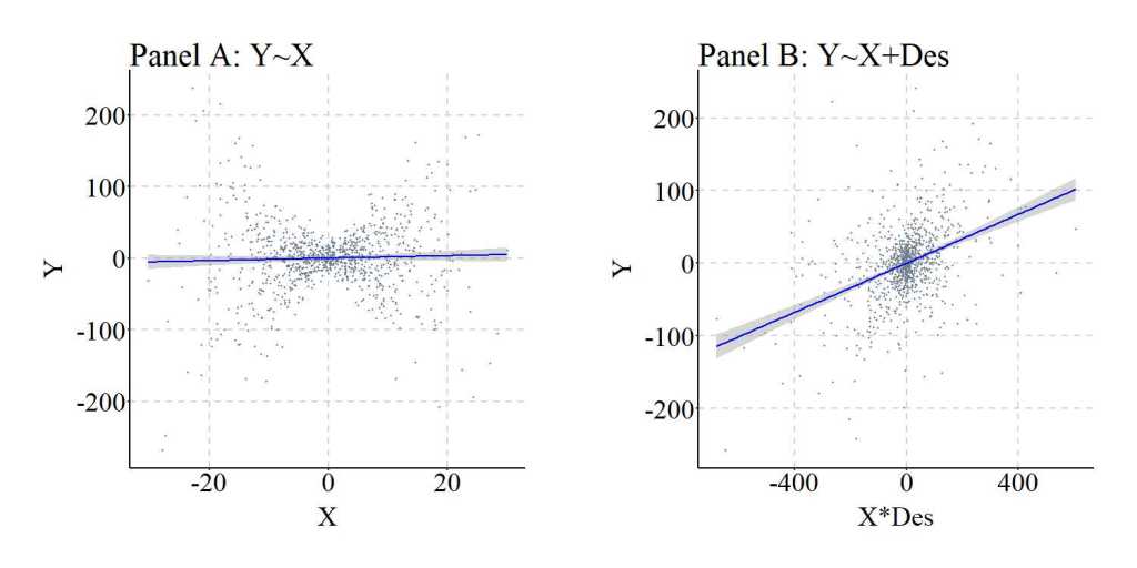
Again, we can replicate this simulation analysis but weaken the causal influence of M on Des.
> ## Example 2 ####
> n<-1000
>
> set.seed(1992)
> X<-rnorm(n,0,10)
> M<-rnorm(n,0,10)
> Y<-0*X+0*M+.5*(X*M)+rnorm(n,0,10)
> Des<-3*M+1*rnorm(n,0,10)
>
> summary(lm(Y~X))

Call:
lm(formula = Y ~ X)

Residuals:
          Min            1Q        Median            3Q           Max
-263.41802778  -20.08017285    0.26256427   21.08051513  242.35063198

Coefficients:
                Estimate   Std. Error  t value Pr(>|t|)
(Intercept) -0.147056842  1.561068597 -0.09420  0.92497
X            0.170546456  0.160141020  1.06498  0.28714

Residual standard error: 49.363555 on 998 degrees of freedom
Multiple R-squared:  0.00113515824,	Adjusted R-squared:  0.000134291665
F-statistic: 1.13417539 on 1 and 998 DF,  p-value: 0.287144056

> lm.beta(lm(Y~X))

Call:
lm(formula = Y ~ X)

Standardized Coefficients::
    (Intercept)               X
0.0000000000000 0.0336921094564

>
> summary(lm(Y~X+Des+X*Des))

Call:
lm(formula = Y ~ X + Des + X * Des)

Residuals:
         Min           1Q       Median           3Q          Max
-87.12503840 -10.88789202  -0.70743204   9.75046825  96.39895051

Coefficients:
                  Estimate     Std. Error  t value             Pr(>|t|)
(Intercept)  0.11494833452  0.61376507350  0.18728              0.85148
X           -0.03038750205  0.06289904139 -0.48312              0.62912
Des         -0.02223004781  0.01961135313 -1.13353              0.25726
X:Des        0.14754988719  0.00200565836 73.56681 < 0.0000000000000002 ***
---
Signif. codes:  0 ‘***’ 0.001 ‘**’ 0.01 ‘*’ 0.05 ‘.’ 0.1 ‘ ’ 1

Residual standard error: 19.3706177 on 996 degrees of freedom
Multiple R-squared:  0.846499566,	Adjusted R-squared:  0.846037215
F-statistic: 1830.86033 on 3 and 996 DF,  p-value: < 0.0000000000000002220446

> lm.beta(lm(Y~X+Des+X*Des))

Call:
lm(formula = Y ~ X + Des + X * Des)

Standardized Coefficients::
      (Intercept)                 X               Des             X:Des
 0.00000000000000 -0.00600316810493 -0.01414348400394  0.91876640659984

>
Discussion & Conclusions
Descendants, conditional upon their ancestors, can reduce or introduce biases into the estimated association between two variables. Under certain circumstances, adjusting for the variation in a descendant can be advantageous. For example, when we can not directly observe the variation associated with a confounder, introducing a descendant of the confounder into a regression model can reduce confounder bias in the estimates corresponding to the association of interest. Additionally, when we can not directly observe variation in a moderator, a descendant of the moderator can permit us to observe how the causal effects of the independent variable on the dependent variable change across scores on the descendant/moderator. Nevertheless, adjusting for the variation in a descendant can also be disadvantageous. For instance, introducing the descendant of collider into a regression model can increase the bias in the estimates corresponding to the association of interest. Alternatively, introducing the descendant of a mediator into a regression model could generate estimates only representative of the direct causal effects. Before concluding, it is important to note with a brief example that adjusting for both the descendant and the ancestor removes the influence of the descendant on the bias within the model (i.e., the ancestor is now the mechanism generating or reducing the bias). This is demonstrated in the syntax below. Given the potential for generating statistical biases and the potential for reducing statistical biases, it is important to identify descendants of key constructs. After identifying the descendants, one can use the principles of Structural Causal Modeling to guide the specification of the regression model and reduce the bias in the estimates produced.
> n<-1000
>
> set.seed(1992)
> Con<-rnorm(n,0,10)
> X<-2*Con+.50*rnorm(n,0,10)
> Y<-2*Con+.00*X+.50*rnorm(n,0,10)
> Des<-20*Con+1*rnorm(n,0,10)
>
>
> summary(lm(Y~X+Con+Des))

Call:
lm(formula = Y ~ X + Con + Des)

Residuals:
          Min            1Q        Median            3Q           Max
-19.618816079  -3.479404832  -0.284815154   3.283236361  16.866716153

Coefficients:
                 Estimate    Std. Error  t value            Pr(>|t|)
(Intercept) -0.0932681968  0.1599235600 -0.58320             0.55989
X           -0.0432234038  0.0323506426 -1.33609             0.18182
Con          2.3392851900  0.3133850695  7.46457 0.00000000000018202 ***
Des         -0.0134316493  0.0153302256 -0.87615             0.38116
---
Signif. codes:  0 ‘***’ 0.001 ‘**’ 0.01 ‘*’ 0.05 ‘.’ 0.1 ‘ ’ 1

Residual standard error: 5.04671047 on 996 degrees of freedom
Multiple R-squared:  0.936520294,	Adjusted R-squared:  0.93632909
F-statistic: 4898.01795 on 3 and 996 DF,  p-value: < 0.0000000000000002220446

> lm.beta(lm(Y~X+Con+Des))

Call:
lm(formula = Y ~ X + Con + Des)

Standardized Coefficients::
     (Intercept)                X              Con              Des
 0.0000000000000 -0.0434986291032  1.1406867662775 -0.1310474314437

>
License: Creative Commons Attribution 4.0 International (CC By 4.0)

One thought on “Entry 10: The Inclusion and Exclusion of Descendants”