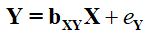
A variety of techniques can be used to simulate linear associations between a continuous independent variable and a normal continuous dependent variable in R. I, however, rely on the lesser employed process of specifying linear directed equations. Briefly, a linear directed equation can be simply thought of as a regression formula but, distinct from when we are estimating a model, we use the equation to indicate causal and non-causal associations. For example, while we can use the equation below to estimate the association between X and Y, we can also use the equation to specify the causal effects of X on Y. Distinct from other simulation techniques, directed equations permits the demarcation of the variance-covariance matrix into causal and non-causal associations.
[Equation 1]
To understand and implement this technique, we must highlight three fundamental principles to specifying directed equation simulations. These principles are listed below:
- The raw value of the modifier (i.e., b or e below) represents the unstandardized slope coefficient for an association.
- The raw value does not provide any information about the amount of variation in the dependent variablecaused by variation in the independent variable.
- The raw value does not provide any information about the standard error of the association.
- If the modifier (i.e., b or e below) is not provided, but variation in a dependent variable is caused by variation in an independent variable, the raw value of the modifier will default to 1.
- The variation in the dependent variable explained by each independent variable or the residual error term is:
- The magnitude of the raw value of the modifier (i.e., b or e below) relative to the magnitude of the raw value of all other modifiers (i.e., b or e below).
- The variation in the independent variable relative to the variation in all other independent variables and residual distributions – determined by specifying the sd values when simulating a continuous construct using rnorm.
- The standard error of an association is:
- The magnitude of the raw value of the modifier (i.e., b or e below) relative to the magnitude of the raw value of all other modifiers (i.e., b or e below).
- The variation in the independent variable relative to the variation in all other independent variables and residual distributions – determined by specifying the sd values when simulating a continuous construct using rnorm.
Now let’s work through some examples to demonstrate how to simulate linear associations between continuous constructs using directed equations. In specification 1, we simulate a linear relationship between X and Y without any other constructs. Given principles 2 and 3, X – in specification 1 – will always predict all of the variation in Y independent of the standard deviation and the raw value of bxy.
[Specification 1]
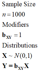
As it can be observed in the syntax below, when we specify the association between X and Y using specification 1, the variation in X perfectly predicts the variation in Y, where a 1 point increase in X corresponds to a 1 point increase in Y. We also get the following warning from R: In summary.lm(lm(Y ~ X)) :essentially perfect fit: summary may be unreliable.
## The Perfect Linear Association ####
> n<-1000 # 1000 cases
>
> ### Modifiers
> bxy<-1
>
> ### Distributions
> set.seed(1992)
> X<-rnorm(n,0,1) # Simulate 1000 scores for X with a mean of 0 and SD of 1
> Y<-bxy*X # Simulate Y = to 1 times
>
> summary(lm(Y~X))

Call:
lm(formula = Y ~ X)

Residuals:
                  Min                    1Q                Median                    3Q
-0.000000000000014681 -0.000000000000000013  0.000000000000000018  0.000000000000000043
                  Max
 0.000000000000000635

Coefficients:
                           Estimate              Std. Error              t value            Pr(>|t|)
(Intercept) -0.00000000000000000351  0.00000000000000001490                -0.24                0.81
X            0.99999999999999955591  0.00000000000000001528 65429659591494184.00 <0.0000000000000002 ***
---
Signif. codes:  0 ‘***’ 0.001 ‘**’ 0.01 ‘*’ 0.05 ‘.’ 0.1 ‘ ’ 1

Residual standard error: 0.000000000000000471 on 998 degrees of freedom
Multiple R-squared:     1,	Adjusted R-squared:     1
F-statistic: 4.28e+33 on 1 and 998 DF,  p-value: <0.0000000000000002

Warning message:
In summary.lm(lm(Y ~ X)) :
  essentially perfect fit: summary may be unreliable
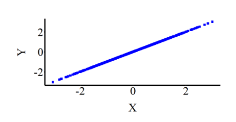
To visually illustrate the association:
Briefly, let’s replicate the first simulation but exclude bxy from the specification to illustrate that the default slope is 1. As demonstrated, the results are identical when the same seed is employed.
> ## The Perfect Linear Association (without Bxy) ####
> n<-1000 # 1000 cases
>
> ### Modifiers
>
> ### Distributions
> set.seed(1992)
> X<-rnorm(n,0,1) # Simulate 1000 scores for X with a mean of 0 and SD of 1
> Y<-X # Simulate Y = to 1 times
>
> summary(lm(Y~X))

Call:
lm(formula = Y ~ X)

Residuals:
                  Min                    1Q                Median                    3Q                   Max
-0.000000000000014681 -0.000000000000000013  0.000000000000000018  0.000000000000000043  0.000000000000000635

Coefficients:
                           Estimate              Std. Error              t value            Pr(>|t|)
(Intercept) -0.00000000000000000351  0.00000000000000001490                -0.24                0.81
X            0.99999999999999955591  0.00000000000000001528 65429659591494184.00 <0.0000000000000002 ***
---
Signif. codes:  0 ‘***’ 0.001 ‘**’ 0.01 ‘*’ 0.05 ‘.’ 0.1 ‘ ’ 1

Residual standard error: 0.000000000000000471 on 998 degrees of freedom
Multiple R-squared:     1,	Adjusted R-squared:     1
F-statistic: 4.28e+33 on 1 and 998 DF,  p-value: <0.0000000000000002

Warning message:
In summary.lm(lm(Y ~ X)) :
  essentially perfect fit: summary may be unreliable
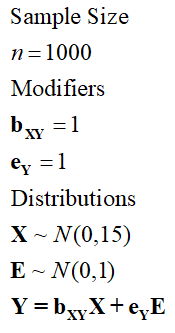
For this next simulation, we want approximately 50 percent of the variation in Y to be caused by variation in X and approximately 50 percent of the variation in Y to be caused by variation in E. E in this example – and all simulation specifications from here on – is used to specify the amount of residual error (or variation) in the dependent variable. When simulating data with multiple dependent variables EYk will be used to represent the residual error term. ey represents the modifier for E. To achieve this, following principles 2 and 3, we want the standard deviation and modifier for X to be identical to the standard deviation and modifier for E (as detailed in Specification 2).
[Specification 2]
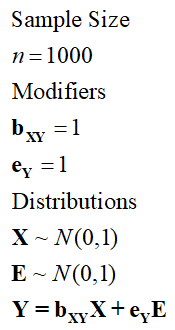
As demonstrated below, although the unstandardized slope coefficients of bXY and eY on Y were both specified to equal 1 and the standard deviation of X and E equaled 1, approximately 49 percent of the variation in Y is explained by X and 51 percent of the variation in Y is explained by E. The amount of variation in Y will never be perfectly evenly explained by variation in X and E due to the probabilistic nature of simulating data. Nevertheless, it can be observed that the identical specification of X and E means that the variation in Y is almost equally caused by both variation in the independent variable (X) and the residual error (E). Importantly, both relationships are statistically significant.
> ## The Linear Association with error term (even effects) ####
> n<-1000 # 1000 cases
>
> ### Modifiers
> bxy<-1
> e<-1
>
> ### Distributions
> set.seed(1992)
> X<-rnorm(n,0,1) # Simulate 1000 scores for X with a mean of 0 and SD of 1
> E<-rnorm(n,0,1) # Simulate 1000 scores for X with a mean of 0 and SD of 1
> Y<-bxy*X+e*E # Simulate Y = to 1 times
>
> summary(lm(Y~X)) # Variation in Y explained by X is the modifier value proportional to the modifiers of all other variables

Call:
lm(formula = Y ~ X)

Residuals:
   Min     1Q Median     3Q    Max
-3.340 -0.639 -0.012  0.677  3.233

Coefficients:
            Estimate Std. Error t value            Pr(>|t|)
(Intercept)   0.0533     0.0312    1.71               0.088 .
X             1.0016     0.0320   31.26 <0.0000000000000002 ***
---
Signif. codes:  0 ‘***’ 0.001 ‘**’ 0.01 ‘*’ 0.05 ‘.’ 0.1 ‘ ’ 1

Residual standard error: 0.988 on 998 degrees of freedom
Multiple R-squared:  0.495,	Adjusted R-squared:  0.494
F-statistic:  977 on 1 and 998 DF,  p-value: <0.0000000000000002

>
> summary(lm(Y~E)) # Variation in Y explained by E (residual Error) is the modifier value proportional to the modifiers of all other variables

Call:
lm(formula = Y ~ E)

Residuals:
    Min      1Q  Median      3Q     Max
-3.0257 -0.6413  0.0076  0.6276  3.0115

Coefficients:
            Estimate Std. Error t value            Pr(>|t|)
(Intercept) -0.00834    0.03090   -0.27                0.79
E            1.00159    0.03127   32.03 <0.0000000000000002 ***
---
Signif. codes:  0 ‘***’ 0.001 ‘**’ 0.01 ‘*’ 0.05 ‘.’ 0.1 ‘ ’ 1

Residual standard error: 0.976 on 998 degrees of freedom
Multiple R-squared:  0.507,	Adjusted R-squared:  0.506
F-statistic: 1.03e+03 on 1 and 998 DF,  p-value: <0.0000000000000002

>
Given principles 2 and 3, if we increase the standard deviation or modifier of X, the variation in Y explained by variation in X will increase. Let’s use Specification 3 – where the SD of X is now equal to 15 – for an example.
[Specification 3]
> ## The Linear Association with error term (sd X = 10*sd E) ####
> n<-1000 # 1000 cases
>
> ### Modifiers
> bxy<-1
> e<-1
>
> ### Distributions
> set.seed(1992)
> X<-rnorm(n,0,15) # Simulate 1000 scores for X with a mean of 0 and SD of 1
> E<-rnorm(n,0,1) # Simulate 1000 scores for X with a mean of 0 and SD of 1
> Y<-bxy*X+e*E # Simulate Y = to 1 times
>
> summary(lm(Y~X)) # Variation in Y explained by X is the modifier value proportional to the modifiers of all other variables

Call:
lm(formula = Y ~ X)

Residuals:
   Min     1Q Median     3Q    Max
-3.340 -0.639 -0.012  0.677  3.233

Coefficients:
            Estimate Std. Error t value            Pr(>|t|)
(Intercept)  0.05328    0.03123    1.71               0.088 .
X            1.00011    0.00214  468.22 <0.0000000000000002 ***
---
Signif. codes:  0 ‘***’ 0.001 ‘**’ 0.01 ‘*’ 0.05 ‘.’ 0.1 ‘ ’ 1

Residual standard error: 0.988 on 998 degrees of freedom
Multiple R-squared:  0.995,	Adjusted R-squared:  0.995
F-statistic: 2.19e+05 on 1 and 998 DF,  p-value: <0.0000000000000002

>
> summary(lm(Y~E)) # Variation in Y explained by E (residual Error) is the modifier value proportional to the modifiers of all other variables

Call:
lm(formula = Y ~ E)

Residuals:
   Min     1Q Median     3Q    Max
-45.39  -9.62   0.11   9.41  45.17

Coefficients:
            Estimate Std. Error t value Pr(>|t|)
(Intercept)   -0.125      0.464   -0.27    0.787
E              1.024      0.469    2.18    0.029 *
---
Signif. codes:  0 ‘***’ 0.001 ‘**’ 0.01 ‘*’ 0.05 ‘.’ 0.1 ‘ ’ 1

Residual standard error: 14.6 on 998 degrees of freedom
Multiple R-squared:  0.00475,	Adjusted R-squared:  0.00375
F-statistic: 4.76 on 1 and 998 DF,  p-value: 0.0293

>
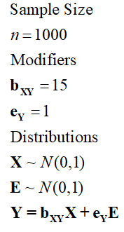
Specification 4, where bXY now equals 15, produces results where X explains the same amount of variation in Y as Specification 3, but the slope of the association is now 15.
[Specification 4]
> ## The Linear Association with error term (bXY = 15*e) ####
> n<-1000 # 1000 cases
>
> ### Modifiers
> bxy<-15
> e<-1
>
> ### Distributions
> set.seed(1992)
> X<-rnorm(n,0,1) # Simulate 1000 scores for X with a mean of 0 and SD of 1
> E<-rnorm(n,0,1) # Simulate 1000 scores for X with a mean of 0 and SD of 1
> Y<-bxy*X+e*E # Simulate Y = to 1 times
>
> summary(lm(Y~X)) # Variation in Y explained by X is the modifier value proportional to the modifiers of all other variables

Call:
lm(formula = Y ~ X)

Residuals:
   Min     1Q Median     3Q    Max
-3.340 -0.639 -0.012  0.677  3.233

Coefficients:
            Estimate Std. Error t value            Pr(>|t|)
(Intercept)   0.0533     0.0312    1.71               0.088 .
X            15.0016     0.0320  468.22 <0.0000000000000002 ***
---
Signif. codes:  0 ‘***’ 0.001 ‘**’ 0.01 ‘*’ 0.05 ‘.’ 0.1 ‘ ’ 1

Residual standard error: 0.988 on 998 degrees of freedom
Multiple R-squared:  0.995,	Adjusted R-squared:  0.995
F-statistic: 2.19e+05 on 1 and 998 DF,  p-value: <0.0000000000000002

>
> summary(lm(Y~E)) # Variation in Y explained by E (residual Error) is the modifier value proportional to the modifiers of all other variables

Call:
lm(formula = Y ~ E)

Residuals:
   Min     1Q Median     3Q    Max
-45.39  -9.62   0.11   9.41  45.17

Coefficients:
            Estimate Std. Error t value Pr(>|t|)
(Intercept)   -0.125      0.464   -0.27    0.787
E              1.024      0.469    2.18    0.029 *
---
Signif. codes:  0 ‘***’ 0.001 ‘**’ 0.01 ‘*’ 0.05 ‘.’ 0.1 ‘ ’ 1

Residual standard error: 14.6 on 998 degrees of freedom
Multiple R-squared:  0.00475,	Adjusted R-squared:  0.00375
F-statistic: 4.76 on 1 and 998 DF,  p-value: 0.0293

>
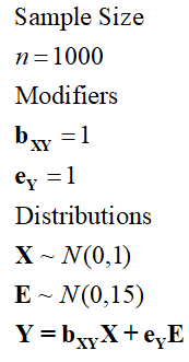
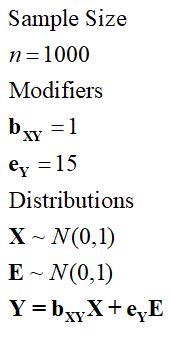
Alternatively, we can change the standard deviation of E or slope of the association between E and Y to influence the variation in Y explained by the variation in X. Take the two examples below:
[Specification 5]
> ## The Linear Association with error term (sd E = 15*sd X) ####
> n<-1000 # 1000 cases
>
> ### Modifiers
> bxy<-1
> e<-1
>
> ### Distributions
> set.seed(1992)
> X<-rnorm(n,0,1) # Simulate 1000 scores for X with a mean of 0 and SD of 1
> E<-rnorm(n,0,15) # Simulate 1000 scores for X with a mean of 0 and SD of 1
> Y<-bxy*X+e*E # Simulate Y = to 1 times
>
> summary(lm(Y~X)) # Variation in Y explained by X is the modifier value proportional to the modifiers of all other variables

Call:
lm(formula = Y ~ X)

Residuals:
   Min     1Q Median     3Q    Max
-50.10  -9.59  -0.19  10.16  48.49

Coefficients:
            Estimate Std. Error t value Pr(>|t|)
(Intercept)    0.799      0.468    1.71    0.088 .
X              1.024      0.481    2.13    0.033 *
---
Signif. codes:  0 ‘***’ 0.001 ‘**’ 0.01 ‘*’ 0.05 ‘.’ 0.1 ‘ ’ 1

Residual standard error: 14.8 on 998 degrees of freedom
Multiple R-squared:  0.00453,	Adjusted R-squared:  0.00354
F-statistic: 4.54 on 1 and 998 DF,  p-value: 0.0333

>
> summary(lm(Y~E)) # Variation in Y explained by E (residual Error) is the modifier value proportional to the modifiers of all other variables

Call:
lm(formula = Y ~ E)

Residuals:
    Min      1Q  Median      3Q     Max
-3.0257 -0.6413  0.0076  0.6276  3.0115

Coefficients:
            Estimate Std. Error t value            Pr(>|t|)
(Intercept) -0.00834    0.03090   -0.27                0.79
E            1.00011    0.00208  479.68 <0.0000000000000002 ***
---
Signif. codes:  0 ‘***’ 0.001 ‘**’ 0.01 ‘*’ 0.05 ‘.’ 0.1 ‘ ’ 1

Residual standard error: 0.976 on 998 degrees of freedom
Multiple R-squared:  0.996,	Adjusted R-squared:  0.996
F-statistic: 2.3e+05 on 1 and 998 DF,  p-value: <0.0000000000000002

>
[Specification 6]
> ## The Linear Association with error term (bXY = 15*e) ####
> n<-1000 # 1000 cases
>
> ### Modifiers
> bxy<-15
> e<-1
>
> ### Distributions
> set.seed(1992)
> X<-rnorm(n,0,1) # Simulate 1000 scores for X with a mean of 0 and SD of 1
> E<-rnorm(n,0,1) # Simulate 1000 scores for X with a mean of 0 and SD of 1
> Y<-bxy*X+e*E # Simulate Y = to 1 times
>
> summary(lm(Y~X)) # Variation in Y explained by X is the modifier value proportional to the modifiers of all other variables

Call:
lm(formula = Y ~ X)

Residuals:
   Min     1Q Median     3Q    Max
-3.340 -0.639 -0.012  0.677  3.233

Coefficients:
            Estimate Std. Error t value            Pr(>|t|)
(Intercept)   0.0533     0.0312    1.71               0.088 .
X            15.0016     0.0320  468.22 <0.0000000000000002 ***
---
Signif. codes:  0 ‘***’ 0.001 ‘**’ 0.01 ‘*’ 0.05 ‘.’ 0.1 ‘ ’ 1

Residual standard error: 0.988 on 998 degrees of freedom
Multiple R-squared:  0.995,	Adjusted R-squared:  0.995
F-statistic: 2.19e+05 on 1 and 998 DF,  p-value: <0.0000000000000002

>
> summary(lm(Y~E)) # Variation in Y explained by E (residual Error) is the modifier value proportional to the modifiers of all other variables

Call:
lm(formula = Y ~ E)

Residuals:
   Min     1Q Median     3Q    Max
-45.39  -9.62   0.11   9.41  45.17

Coefficients:
            Estimate Std. Error t value Pr(>|t|)
(Intercept)   -0.125      0.464   -0.27    0.787
E              1.024      0.469    2.18    0.029 *
---
Signif. codes:  0 ‘***’ 0.001 ‘**’ 0.01 ‘*’ 0.05 ‘.’ 0.1 ‘ ’ 1

Residual standard error: 14.6 on 998 degrees of freedom
Multiple R-squared:  0.00475,	Adjusted R-squared:  0.00375
F-statistic: 4.76 on 1 and 998 DF,  p-value: 0.0293

>
Using the principles above, you can now simulate linear associations with normal continuous variables. We will continue reviewing the basics of simulating data in the next entry covering the process of simulating linear associations with a categorical variables.
