When I state “X is a cause of Y”, I am inherently implying that variation in X caused variation in Y. This statement, however, does not provide any indication of how X caused variation in Y. The how is just as important, if not more important, than knowing the causal association. Take for example the statement “genetics cause cancer”. Well, genetics are causally related to cancer, but that causal relationship is extremely complicated. Variation in your genetic code can directly cause variation in cancer by creating an increased predisposition to cellular mutations, variation in your genetic code can indirectly cause variation in cancer by creating variation in environmental factors, or variation in your genetic code can directly or indirectly only cause variation in cancer in the presence of certain environmental factors. The total causal pathway between any X and Y can be broken down into the: (1) direct causal pathway, (2) indirect causal pathway, (3) direct causal pathway under certain conditions, and (4) indirect causal pathway under certain conditions.
The causal pathway of interest, inherent in our hypotheses and research questions, generates assumptions about what the coefficients in a regression model represent. For example, if I state “it is hypothesized that gene XX causes an increased risk of cancer” I am intrinsically stating my interest in the total causal effects of gene XX on cancer. Here, assuming the association is not confounded, I can simply estimate the bivariate association. However, if I state that “it is hypothesized that gene XX causes an increased risk of cancer through dietary habits” I am implicitly interested in the indirect causal effects of gene XX on cancer. Estimating a regression model of the bivariate association between gene XX and cancer does not produce coefficients representative of the indirect causal effects. Similarly, if I state that “it is hypothesized that gene XX directly causes an increased risk of cancer”, my regression model would have to adjust for the variation in any indirect pathway to ensure the coefficients only represent the direct causal pathway. Evident by the examples, the manner in which we state our hypotheses and research questions generates an assumption about what causal pathway the produced coefficients represent. If the model is accidentally misspecified, the observed coefficients will not represent the causal pathway of interest and, in turn, violate the assumptions within our hypotheses. But before illustrating this principal, let’s discuss the distinction between the causal pathways.
Causal Pathways
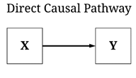
As introduced above, four unique causal pathways can theoretically exist between two constructs, the direction and magnitude of which contributes to the direction and magnitude of the total causal pathway. Let’s start with the easiest, the direct causal pathway. For a direct causal pathway to exist no other mechanism can mediate the relationship between the input – or independent variable – and the outcome – or the dependent variable. For example, the golf head speed and location of a swing for Brooks Koepka – team Koepka all the way! – is a direct cause of the distance a golf ball traveled. Importantly, while this example is immediate in time, a direct causal pathway does not have any time requirements, only the requirement that no mechanism mediates the association. Direct causal pathways not immediate in time, however, are uncommon within the social sciences.
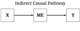
An indirect causal pathway is the combination of multiple direct causal pathways. For example, an indirect causal pathway with one mediator exists when variation in a distant input causes variation in an intermediate mechanism (the first direct causal pathway) and variation in the intermediate mechanism causes variation in an outcome (the second direct causal pathway). The intermediate mechanism serves as a mediator, where the indirect causal effects of the input on the outcome exists as a product of the mediator. In theory, an infinite number of mediators can exist within an indirect causal pathway. To provide an example, genetics has an indirect causal pathway to human behavior through a host of mechanisms including, but not limited to, brain development, hormone production, environmental selection, and psychological functioning. Moreover, to revert back to a sports example, Aaron Rodgers training has an indirect causal effect on how he performs in a game, through his muscle memory, knowledge of the defense, muscle fatigue, and etc. Again, similar to direct causal pathways, indirect causal pathways do not have any time requirements and can occur in extremely short periods of time. For instance, electric signals in one neuron indirectly cause electric signals in another neuron through the release and uptake of chemicals within the synapse, all of which happens in the span of milliseconds.
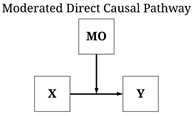
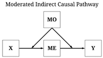
A moderated direct causal pathway exists when the magnitude, direction, or existence of a direct causal pathway differs in the presence of one or more mechanisms. To revert back to the golf example, while the golf head speed and location of a swing directly causes the distance a golf ball travels, the effects vary by the air quality, humidity, temperature, windspeed, and etc. Similarly, a moderated indirect causal pathway exists when the magnitude, direction, or existence of an indirect causal pathway differs in the presence of one or more mechanisms. Explicitly, this means that an indirect causal pathway can become a moderated indirect causal pathway when the magnitude, direction, or existence of one or more direct pathways vary by the presence of an external mechanism. For instance, Aaron Rodgers training has an indirect causal effect on how he performs in a game, but that effect of fatigue on how he performs differs by air quality, humidity, temperature, windspeed, and how well everyone around him is playing.
Each of these causal pathways can exist simultaneously, generating the observation of unique causal effects between X and Y depending upon how a regression model is estimated. As such, it is important to theoretically consider how X causes variation in Y preceding the estimation of any regression model.
Estimating the Causal Effects of Each Pathway
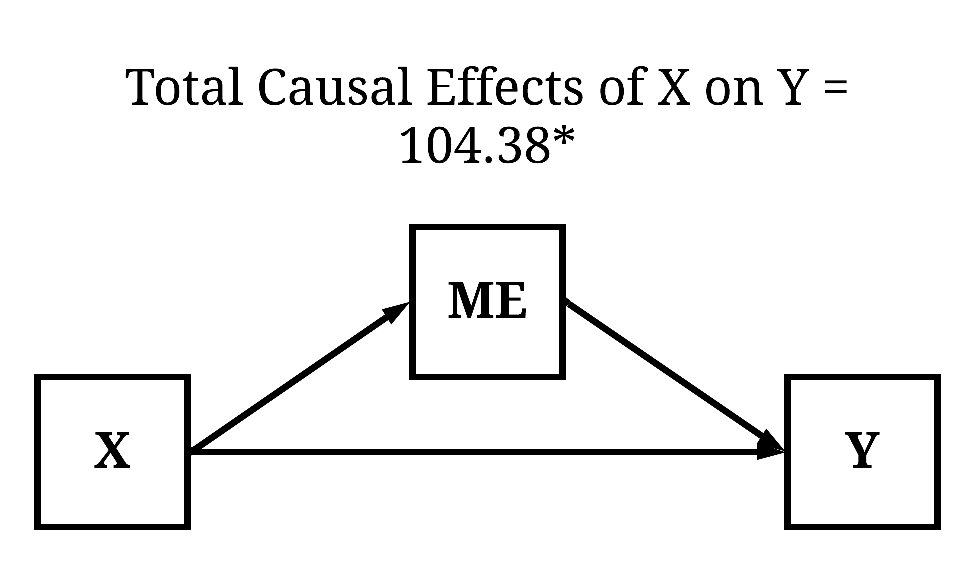
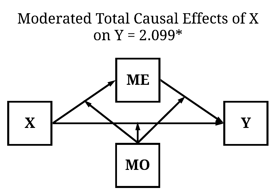
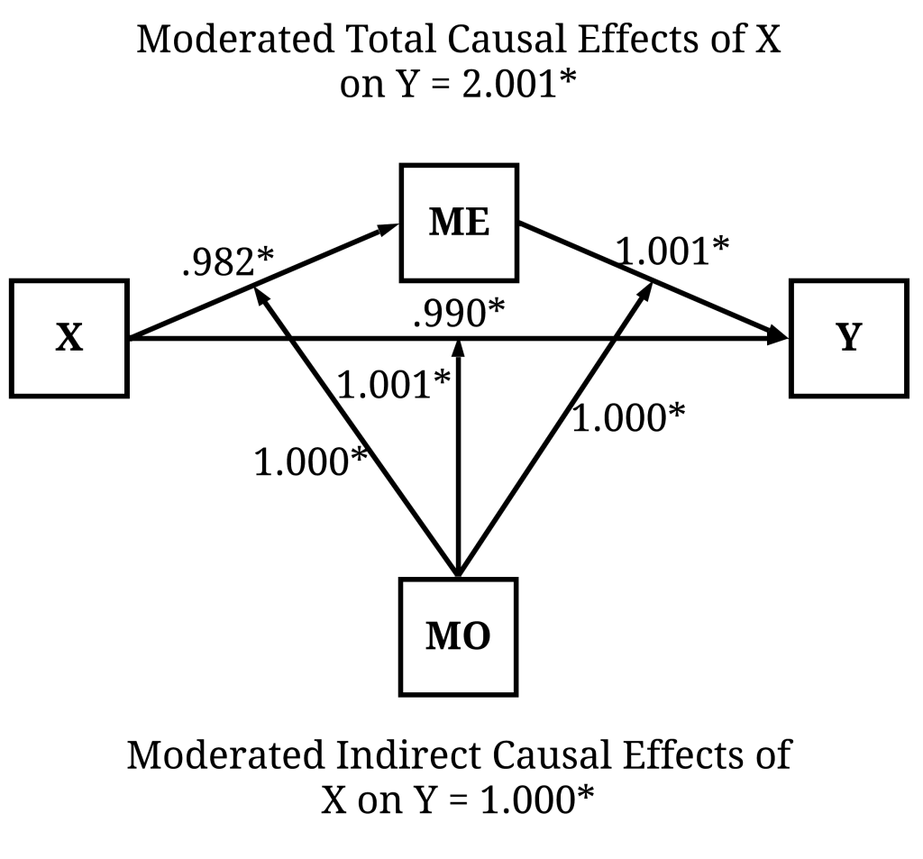
For the purposes of the current demonstration, the data simulation will specify that the total causal effects of X on Y is a combination of all of the causal pathways that can exist. Explicitly, following the diagram below, a direct causal effect and an indirect causal effect – through ME – were specified to exist from X to Y, the effects of which are moderated by scores on MO. The employment of a single structural causal network permits us to generate estimates for all of the causal effects of X on Y, as well as illustrate the differences between the causal estimates.
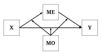
Following our reliance on directed equation simulations, the data was simulated using the syntax below. Briefly, X and MO were specified as normally distributed variables with a mean of 0 and a standard deviation of 10. Variation in ME was specified to be directly causally influenced by variation in X and random error with a mean of 0 and a standard deviation of 10. The magnitude of the direct causal effects of X on ME was moderated by scores on MO. Similarly, variation in Y was specified to be directly causally influenced by variation in X, variation in ME, and random error with a mean of 0 and a standard deviation of 10. The magnitude of the direct causal effects of X and ME on Y, however, was specified to be moderated by scores on MO.
set.seed(1992)
n<-10000 # Sample Size
X<-rnorm(n,0,10) # Independent Variable
MO<-rnorm(n,0,10)
ME<-1.00*X+1.00*(X*MO)+2.00*rnorm(n,0,10) # Mediator Variable
Y<-1.00*ME+1.00*(ME*MO)+1.00*X+1.00*(X*MO)+2.00*rnorm(n,0,10) # Dependent Variable

DF<-data.frame(X,MO,ME,Y)
Total Causal Effects (Unconditional)
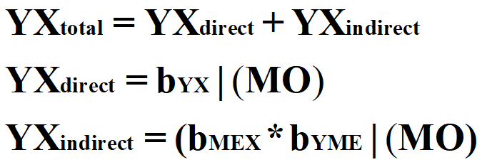
Now let’s estimate some effects, starting with the unconditional total causal effects. The total unconditional causal effects represent the combination of all of the effects of X on Y and is calculated using the equations below.[i] Explicitly, the unconditional total causal effect of X on Y is equal to the direct causal effect of X on Y plus the indirect causal effect of X on Y. The direct causal effect of X on Y is the value of bYX across the entire distribution of MO, while the indirect causal effects of X on Y is bMEX multiplied by BYME across the entire distribution of MO.
[Equation 1]
To observe the unconditional total causal effects, we can simply estimate a bivariate OLS regression model of Y on X. Evident by the findings, a 1 point increase in X causes a 104.378 increase in Y (β = .557).
> summary(lm(Y~X, data = DF))

Call:
lm(formula = Y ~ X, data = DF)

Residuals:
         Min           1Q       Median           3Q          Max
-36956.51320   -492.65349     10.91097    506.05138  27639.21191

Coefficients:
                Estimate   Std. Error  t value             Pr(>|t|)
(Intercept) -17.58947245  15.57680124 -1.12921              0.25884
X           104.37890336   1.55709982 67.03418 < 0.0000000000000002 ***
---
Signif. codes:  0 ‘***’ 0.001 ‘**’ 0.01 ‘*’ 0.05 ‘.’ 0.1 ‘ ’ 1

Residual standard error: 1557.54009 on 9998 degrees of freedom
Multiple R-squared:  0.310082167,	Adjusted R-squared:  0.310013161
F-statistic: 4493.58076 on 1 and 9998 DF,  p-value: < 0.0000000000000002220446

> lm.beta(lm(Y~X, data = DF))

Call:
lm(formula = Y ~ X, data = DF)

Standardized Coefficients::
   (Intercept)              X
0.000000000000 0.556850219132

>
Total Causal Effects (Moderated)
The simplest way to calculate the conditional total causal effects is to regress Y on X at specific values of MO. For example, using the following equation, we can calculate the total causal effects of X on Y when MO is greater than 1 SD away from the mean.
[Equation 2]
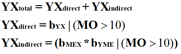
By estimating the OLS regression model of Y on X with only cases that had a value on MO > 10, a unique estimate for the total causal effects of X on Y is produced. Specifically, for cases with values on MO > 10, a 1 point increase in X causes a 296.721 increase in Y (β = .843). Given that MO is a continuous construct, we can calculate conditional total causal effects of X on Y across the entire distribution of MO – we, however, won’t do that because it requires the estimation of numerous regression models.
> summary(lm(Y~X, data = DF[which(DF$MO>10),]))

Call:
lm(formula = Y ~ X, data = DF[which(DF$MO > 10), ])

Residuals:
          Min            1Q        Median            3Q           Max
-17755.378780   -665.205154    -22.661785    664.391620  22361.476927

Coefficients:
                Estimate   Std. Error  t value            Pr(>|t|)
(Intercept)   2.71454150  48.41920601  0.05606              0.9553
X           296.72099681   4.78082742 62.06478 <0.0000000000000002 ***
---
Signif. codes:  0 ‘***’ 0.001 ‘**’ 0.01 ‘*’ 0.05 ‘.’ 0.1 ‘ ’ 1

Residual standard error: 1919.41272 on 1571 degrees of freedom
Multiple R-squared:  0.710309913,	Adjusted R-squared:  0.710125514
F-statistic: 3852.03679 on 1 and 1571 DF,  p-value: < 0.0000000000000002220446

> lm.beta(lm(Y~X, data = DF[which(DF$MO>10),]))

Call:
lm(formula = Y ~ X, data = DF[which(DF$MO > 10), ])

Standardized Coefficients::
   (Intercept)              X
0.000000000000 0.842798856595

>
Instead, we can calculate the conditional total causal effects of X on Y by regressing Y on X, MO, and an interaction between MO and X. Ignoring the direct estimates – they provide limited value in an interaction model –, the interaction between MO and X indicates that as scores on X increase and scores on MO increase the magnitude of the total causal effects of X on Y becomes stronger to a degree of 2.099 (b = 2.099, β = .152).
> summary(lm(Y~X+MO+(X*MO), data = DF))

Call:
lm(formula = Y ~ X + MO + (X * MO), data = DF)

Residuals:
         Min           1Q       Median           3Q          Max
-39002.57746   -478.66599     26.09335    499.73783  28115.66175

Coefficients:
                 Estimate    Std. Error  t value               Pr(>|t|)
(Intercept) -20.934662684  15.423450011 -1.35733                0.17471
X           104.370148587   1.541756629 67.69561 < 0.000000000000000222 ***
MO            6.171780872   1.541903304  4.00270            0.000063075 ***
X:MO          2.099475702   0.152219126 13.79246 < 0.000000000000000222 ***
---
Signif. codes:  0 ‘***’ 0.001 ‘**’ 0.01 ‘*’ 0.05 ‘.’ 0.1 ‘ ’ 1

Residual standard error: 1541.92432 on 9996 degrees of freedom
Multiple R-squared:  0.323982194,	Adjusted R-squared:  0.323779307
F-statistic: 1596.86425 on 3 and 9996 DF,  p-value: < 0.0000000000000002220446

> lm.beta(lm(Y~X+MO+(X*MO), data = DF))

Call:
lm(formula = Y ~ X + MO + (X * MO), data = DF)

Standardized Coefficients::
    (Intercept)               X              MO            X:MO
0.0000000000000 0.5568035133416 0.0329230065591 0.1134284720746

>
Direct Causal Pathway (Unconditional)
We can calculate the unconditional direct causal effects of X on Y by removing the unconditional indirect causal effect between X and Y. This can be achieved by adjusting the regression model of Y on X for the variation in ME. To briefly explain why this works, let’s make some logic statements about the data:
The variation in ME can be broken down into two parts:
(1) Variation directly caused by X
(2) Variation caused by random error
The variation in Y can be broken down into three parts:
(1) Variation directly caused by X
(2) Variation directly caused by ME
(3) Variation caused by random error
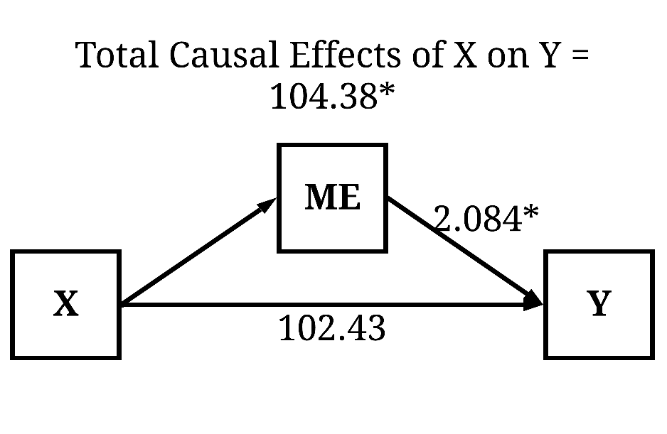
Using these statements, it is logical that some of the variation in ME is caused by variation in X and causes variation in Y. This shared variation between the three constructs is the unconditional indirect causal pathway. By simply introducing ME as a statistical control, the variation in Y directly caused by ME is removed – including the variation shared between the three constructs – from the estimated association between X and Y, permitting the slope coefficient to only represent the unconditional direct causal effects. But let’s see our estimates. As it can be observed, the unconditional direct causal effects of X on Y is 102.434 (β = .546).
> summary(lm(Y~X+ME, data = DF))

Call:
lm(formula = Y ~ X + ME, data = DF)

Residuals:
         Min           1Q       Median           3Q          Max
-39229.61629   -476.95047     20.82690    498.69863  27816.06452

Coefficients:
                 Estimate    Std. Error  t value             Pr(>|t|)
(Intercept) -20.288729973  15.429626706 -1.31492              0.18857
X           102.434803473   1.548561553 66.14836 < 0.0000000000000002 ***
ME            2.084127472   0.149536892 13.93721 < 0.0000000000000002 ***
---
Signif. codes:  0 ‘***’ 0.001 ‘**’ 0.01 ‘*’ 0.05 ‘.’ 0.1 ‘ ’ 1

Residual standard error: 1542.70242 on 9997 degrees of freedom
Multiple R-squared:  0.323232051,	Adjusted R-squared:  0.323096657
F-statistic: 2387.34032 on 2 and 9997 DF,  p-value: < 0.0000000000000002220446

> lm.beta(lm(Y~X+ME, data = DF))

Call:
lm(formula = Y ~ X + ME, data = DF)

Standardized Coefficients::
   (Intercept)              X             ME
0.000000000000 0.546478655382 0.115141018013

>
Direct Causal Pathway (Moderated)
Similar to the preceding example, to estimate the conditional direct causal effects of X on Y we have to condition the entire equation upon MO. That is, we need to include an interaction term between X and MO, and an interaction term between ME and MO to observe an estimate representative of the conditional direct causal effects of X on Y. Take a second and guess what the estimate will be? If you guessed it will be ~ 1.00, you must’ve payed attention to the process used to simulate the data. Explicitly, the estimation below employs the formula used to create variation in Y, which approximately reproduces the estimates used to simulate the data.
> summary(lm(Y~X+ME+MO+(X*MO)+(MO*ME), data = DF))

Call:
lm(formula = Y ~ X + ME + MO + (X * MO) + (MO * ME), data = DF)

Residuals:
         Min           1Q       Median           3Q          Max
-71.52270176 -13.74040107  -0.04610956  13.56569193  69.35878533

Coefficients:
                   Estimate      Std. Error    t value             Pr(>|t|)
(Intercept)  0.087740584106  0.199775785840    0.43920              0.66053
X            0.989644628777  0.025885238207   38.23201 < 0.0000000000000002 ***
ME           1.001267146613  0.010095571104   99.17885 < 0.0000000000000002 ***
MO          -0.029651948625  0.019980866923   -1.48402              0.13784
X:MO         1.001169783134  0.010281344249   97.37732 < 0.0000000000000002 ***
ME:MO        1.000064148382  0.000129552884 7719.35071 < 0.0000000000000002 ***
---
Signif. codes:  0 ‘***’ 0.001 ‘**’ 0.01 ‘*’ 0.05 ‘.’ 0.1 ‘ ’ 1

Residual standard error: 19.9638423 on 9994 degrees of freedom
Multiple R-squared:  0.999886699,	Adjusted R-squared:  0.999886642
F-statistic: 17639519.8 on 5 and 9994 DF,  p-value: < 0.0000000000000002220446

> lm.beta(lm(Y~X+ME+MO+(X*MO)+(MO*ME), data = DF))

Call:
lm(formula = Y ~ X + ME + MO + (X * MO) + (MO * ME), data = DF)

Standardized Coefficients::
       (Intercept)                  X                 ME                 MO               X:MO
 0.000000000000000  0.005279647616876  0.055316634951478 -0.000158176597529  0.054090246754991
             ME:MO
 0.987820735912706

>
Indirect Causal Pathway (Unconditional)
Although separate regression models can be estimated to calculate indirect causal pathways, the easiest process is through the implementation of path analysis. Path analysis – to quickly introduce – is a method in which regression equations are stacked on top of one another (or plugged into one another).[ii] Although not directly observed, the logic and process of specifying a path model is the same logic and process we use to conduct our simulations (directed equations). In this circumstance and anytime we estimate a path model in this series, we will use Lavaan. Since we are working with non-clustered continuous constructs, the Maximum Likelihood estimator in Lavaan works best.
To estimate the indirect effects in Lavaan, we will specify two equations within F1 – our formula. Within F1, we regress (Eq.1) ME on X and (Eq.2) Y on ME and X. The letters a, b, and c inform Lavaan to save the unstandardized slope coefficient as the corresponding letter, which we then use to calculate the indirect effects and total effects. To calculate the indirect effects, the slope coefficient of the association between ME and X (saved as b) is multiplied by the association between Y and ME. The total effects, consistent with our discussion above, is calculated by adding the slope of the direct association between Y and X to the indirect calculation.
>F1<-'
>ME~b*X
>Y~c*ME+a*X
>
>bc:=b*c
>abc:=(b*c)+a
>
>'
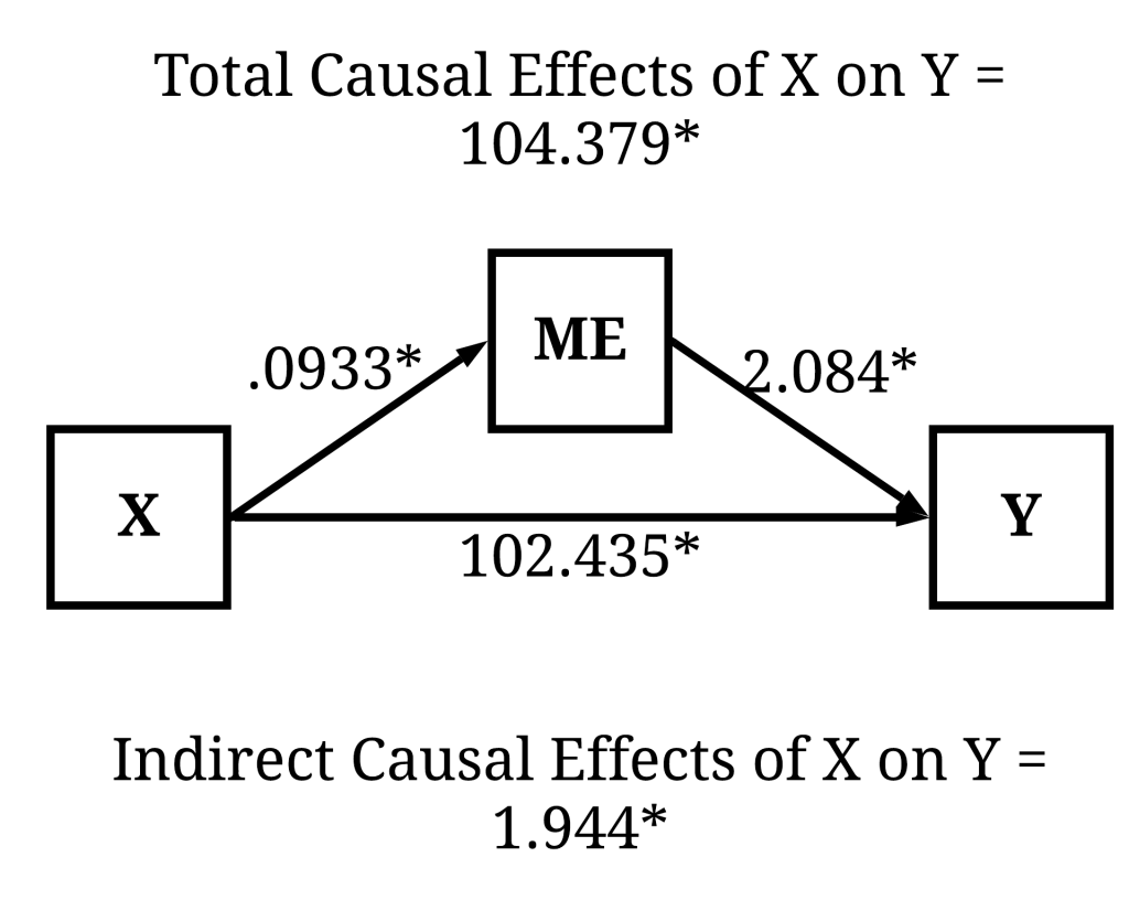
Once we specify our formula, we can estimate the path model in Lavaan using the sem command with the ML estimator. To simplify the output, only the regression estimates and the defined parameters are presented here. You can see the full Lavaan output if you estimate the association using the provided R-code. Focusing on key estimates, it can be observed that the direct effects of X on Y (labeled with a) is almost identical to the estimate produced above. The indirect slope coefficient of X on Y through ME (bc within the defined parameters section) is 1.944, which has a standardized effect of β = .010. The total slope coefficient of X on Y (abc within the defined parameters section) – which is identical to regressing Y on X – is 104.379, which has a standardized effect of β = .557. As a brief note, the significance of the defined parameters in Lavaan is calculated using the delta method.
>M1<-sem(F1, data=DF , estimator = "ML")
>summary(M1, standardized = TRUE, ci = TRUE, rsquare = T)

Regressions:
                   Estimate     Std.Err   z-value  P(>|z|) ci.lower    ci.upper      Std.lv     Std.all
  ME ~
    X          (b)       0.933     0.103    9.044    0.000       0.731       1.135       0.933    0.090
  Y ~
    ME         (c)       2.084     0.150   13.939    0.000       1.791       2.377       2.084    0.115
    X          (a)     102.435     1.548   66.158    0.000      99.400     105.469     102.435    0.546


Defined Parameters:
                   Estimate     Std.Err   z-value  P(>|z|) ci.lower    ci.upper      Std.lv     Std.all
    bc                   1.944     0.256    7.587    0.000       1.442       2.446       1.944    0.010
    abc                104.379     1.557   67.041    0.000     101.327     107.430     104.379    0.557
Indirect Causal Pathway (Moderated)
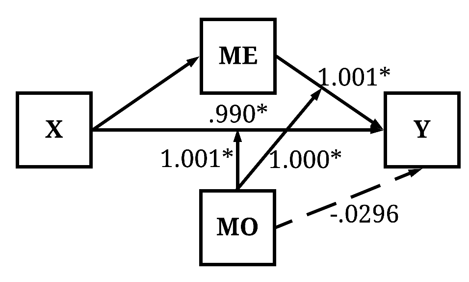
To calculate the moderated indirect causal pathways, we first have to create XMO (specified as X*MO) and MEMO (ME*MO) because Lavaan does not permit the specification of interaction terms within the formula (e.g., the way the interactions were specified when using the lm command). Focusing on the moderated indirect effects, it can be observed that the effects of X on Y through ME conditional on MO is equal to 1.000. Take a second and identify the rest of the causal effects of X on Y observed below.
DF$XMO<-DF$X*DF$MO
DF$MEMO<-DF$ME*DF$MO

F1<-'
ME~X+MO+b*(XMO)
Y~ME+MO+c*(MEMO)+X+a*(XMO)

bc:=b*c
abc:=(b*c)+a

'

Regressions:
                   Estimate     Std.Err  z-value  P(>|z|) ci.lower    ci.upper      Std.lv     Std.all
  ME ~
    X                    0.982    0.020   49.663    0.000       0.943       1.021       0.982    0.095
    MO                  -0.019    0.020   -0.980    0.327      -0.058       0.019      -0.019   -0.002
    XMO        (b)       1.000    0.002  511.980    0.000       0.996       1.003       1.000    0.977
  Y ~
    ME                   1.001    0.010   99.214    0.000       0.981       1.021       1.001    0.055
    MO                  -0.030    0.020   -1.484    0.138      -0.069       0.009      -0.030   -0.000
    MEMO       (c)       1.000    0.000 7722.066    0.000       1.000       1.000       1.000    0.988
    X                    0.990    0.026   38.168    0.000       0.939       1.040       0.990    0.005
    XMO        (a)       1.001    0.010   97.410    0.000       0.981       1.021       1.001    0.054

Defined Parameters:
                   Estimate     Std.Err  z-value  P(>|z|) ci.lower    ci.upper      Std.lv     Std.all
    bc                   1.000    0.002  510.858    0.000       0.996       1.003       1.000    0.966
    abc                  2.001    0.010  191.235    0.000       1.980       2.021       2.001    1.020
Discussion & Conclusion
So you might be asking, what does this have to do with assumption violations? This is a great question, which I ask you to think about the research process. When we estimate a regression model, we generally follow the guidance of a hypothesis or research question. For instance, it is hypothesized that a felony conviction decreases the ability to obtain a job. Although not explicit, the manner in which this hypothesis is stated generates an assumption that we are interested in the total causal effects of a felony conviction on employment. Similarly, if we stated it is hypothesized that a felony conviction decreases the ability to obtain a job through the inability to find transportation it is assumed that we are interested in the indirect causal effects of a felony conviction on employment. The assumptions inherent in our stated hypotheses possess important implications for the specification of a regression model, where alternative specifications could produce estimates not representative of the causal effects of interest.
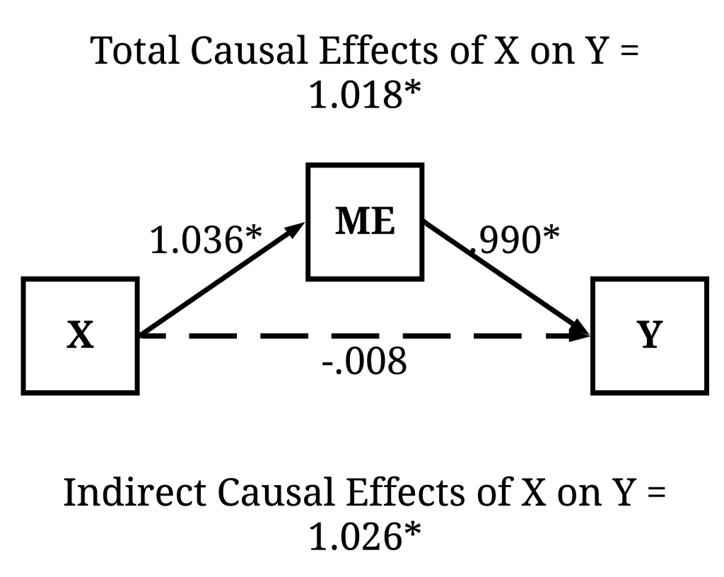
To provide an example, let’s focus on a simulation without a moderating effect and no-direct effect of X on Y. Within this specification, variation in X only indirectly causes variation in Y. This means that X does cause variation in Y (i.e., the total causal effects), but only through ME.
> set.seed(1992)
> n<-10000 # Sample Size
> X<-rnorm(n,0,10) # Independent Variable
> ME<-1.00*X+2.00*rnorm(n,0,10) # Mediator Variable
> Y<-1.00*ME+0*X+2.00*rnorm(n,0,10) # Dependent Variable
>
> DF<-data.frame(X,ME,Y)
>
Now imagine we are interested in the total causal effects of X on Y. As presented in the results below, the total causal effects of X on Y is statistically significant (p < .001), suggesting that a 1 point increase in X corresponds to a 1.018 increase in Y (abc within the defined parameters section). The observed coefficients, as demonstrated above, is identical to regressing Y on X without any statistical controls. These results would be interpreted as variation in X causally influences variation in Y.
Now, imagine we regressed Y on X but accidentally included ME as a statistical control. The inclusion of ME as a statistical control adjusts the regression estimates, where the observed coefficients of the effects of X on Y only represent the direct causal effects. In this example, consistent with the results presented below, variation in X does not directly cause variation in Y. As such, the accidental inclusion of ME in the regression analysis would generate the interpretation – if we are only interested in the total causal effects – that variation in X does not causally influence variation in Y. This interpretation, however, only exists because the estimated coefficients represent the direct causal effects – not the total causal effects –, which occurred because ME was included as a covariate in the regression model. As such, the statistical coefficient violates the assumption stated within our hypothesis or research question.
F1<-'
ME~b*X
Y~c*ME+a*X

bc:=b*c
abc:=(b*c)+a

'

M1<-sem(F1, data=DF , estimator = "ML")
summary(M1, standardized = TRUE, ci = TRUE, rsquare = T)

Regressions:
                   Estimate  Std.Err  z-value  P(>|z|) ci.lower ci.upper   Std.lv  Std.all
  ME ~
    X          (b)    1.036    0.020   51.817    0.000    0.997    1.075    1.036    0.460
  Y ~
    ME         (c)    0.990    0.010  100.158    0.000    0.971    1.010    0.990    0.749
    X          (a)   -0.008    0.022   -0.372    0.710   -0.052    0.035   -0.008   -0.003

Defined Parameters:
                   Estimate  Std.Err  z-value  P(>|z|) ci.lower ci.upper   Std.lv  Std.all
    bc                1.026    0.022   46.023    0.000    0.982    1.070    1.026    0.345
    abc               1.018    0.028   36.373    0.000    0.963    1.073    1.018    0.342
The assumption violation does not come from the estimated association, but rather is a product of our initial research question and the process used to interpret the estimate. To avoid this violation, it is always important to: (1) define the causal effects of interest (total, direct, or indirect), (2) theorize about and identify potential mediators and moderators using the principles of structural causal modeling (Pearl, 2009), (3) properly specify the regression equation to accurately estimate the causal effects of interest. Through this process you will produce statistical coefficients representative of the causal effects of interest to you!
[i] I know I generally avoid formulas in this series, but it is really important to know how each of these effects is calculated.
[ii] A more detailed discussion of path analysis will be provided in later entries.

2 thoughts on “Entry 9: The Inclusion and Exclusion of Mediating and Moderating Mechanisms”