You might be saying that Entry 7 provides good evidence for why we should include numerous variables in a statistical model and hope they adjust for confounder bias. I mean… in some sense… climate change can confound the association between unemployment rates and crime rates. While it does suggest that, it would be negligent for me to recommend adjusting our estimates for any variable that is empirically related to the independent and dependent variable of interest. This is because any of the variables we introduce into our statistical model could function as a collider. And, opposite of a confounder, when a collider variable is introduced into a multivariable model, it can bias the estimated association between the independent and dependent variable of interest.
Collider Variables
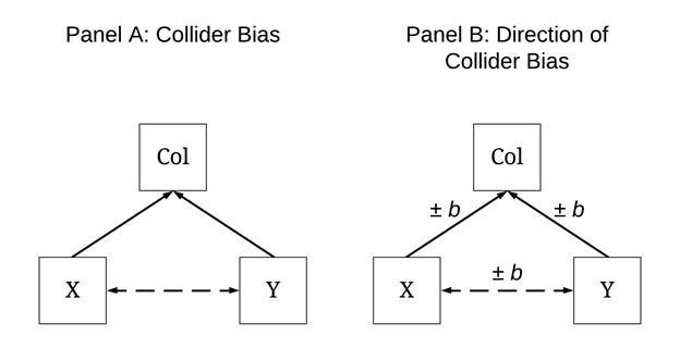
It is important to develop an understanding of what a collider variable is before illustrating the effects of collider variables in multivariable models. A collider variable is the opposite of a confounder, where variation in the Col is caused by both variation in X and variation in Y (illustrated below). For example, it can be suspected that both professional appearance during a job interview and educational attainment (e.g., degree earned) can causally influence the likelihood of an individual being employed (i.e., a collider). Assuming that professional appearance during a job interview has no effect on educational attainment, estimating the bivariate association will produce estimates consistent with the null association. Nevertheless, if we estimated a multivariable model adjusting for the influence of being employed – the theorized collider –, the slope coefficient of the association between professional appearance during a job interview and educational attainment will become biased. That is, adjusting for the influence of a collider in a multivariable model will bias the observed association between the variables of interest. Similar to confounder bias, the direction and the magnitude of the collision dictate the direction and magnitude of the bias in the slope coefficient. As such, conditional upon the true association, adjusting a multivariable model for the influence of a collider can generate Type 1, Type 2, Type M (magnitude biases), and Type S errors (slope coefficients with signs opposite of the true association).
Important Note: Identifying a Collider – Good Luck!
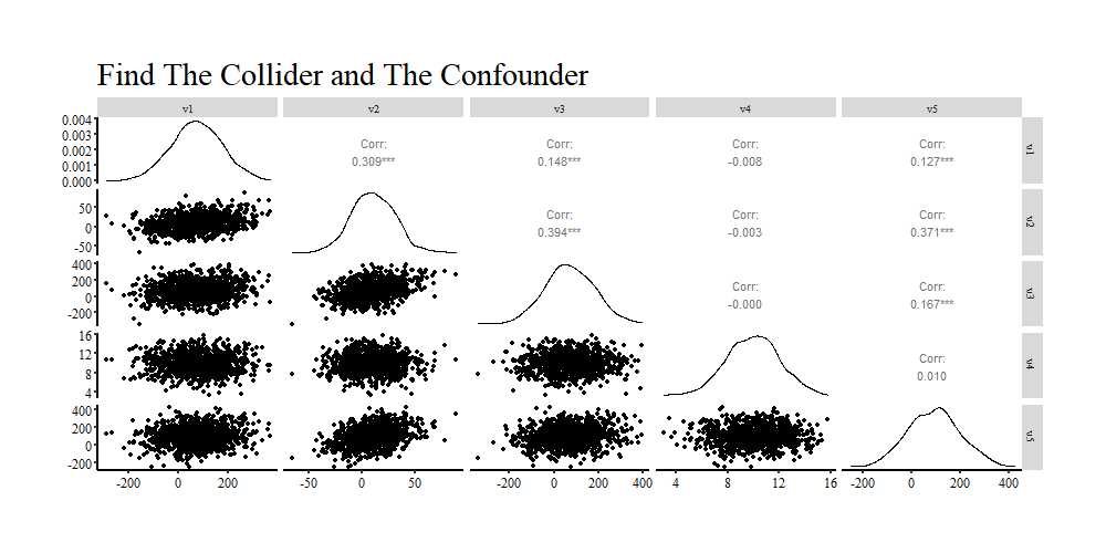
So… in the previous entry we did not discuss the variety of statistical techniques used to identify a confounder between an independent and dependent variable. This is because scholars commonly rely on bivariate statistics to identify potential confounders. This is not an appropriate technique for a variety of reasons – including variables can become confounders only within the context of a multivariable model (this will be discussed in future entries) –, but the primary reason is that colliders and confounders look extremely similar in correlation matrices and other bivariate statistics. Look at the figure below and (1) identify the relationship confounded and which variable is confounding the association?, as well as (2) identify the collider and the two variables causing variation in the collider? Any ideas? I bet you thought V3 is the collider between V1 and V2… hmm, though V5 is related to every variable? If you can correctly identify both the confounder and the collider from a correlation matrix you have a super power and should monetize that immediately! For the rest of us, identifying the confounders and colliders requires a sound theoretical model and a directed acyclic graph (DAG). While the stepwise estimation of regression models including and excluding every variable (one at a time) might appear to be a valid technique for identifying confounders and colliders, be careful as you could end up p-hacking a model.
True Association Between X and Y = 0
Consistent with the entire series, we will conduct simulation analyses to evaluate the direction (upwardly or downwardly) and magnitude of the bias in the slope coefficient between X and Y when the association is conditioned – or adjusted for – the influence of a collider. For the first set of simulations, we will specify that the independent variable (X) and dependent variable (Y) are unrelated. That is, variation in X does not cause variation in Y and the slope of the association between the variables is 0 (i.e., b = 0). Notably, while these simulations will be very similar to entry 7, X and Y will now causally influence variation in the collider.
Collider (+,+)
Let’s start the simulations by having variation in the independent variable (X) and variation in the dependent variable (Y) causally predict variation in the collider. To begin the specification, we simulate two normally distributed variables – using separate seeds – with a mean of 0 and a standard deviation of 2.5. The first variable we will label as X, while the second variable will be labeled as Y. Additionally, each variable will be specified to have 500 cases. After simulating X and Y, we can specify that C – the collider – is equal to 2*X plus 2*Y with a normally distributed residual variation specified to have a mean of 0 and a standard deviation of 2.5. This specification means that a 1-point increase in X and Y is associated with a 2-point increase in C. Importantly, as specified the true association between X and Y is not statistically significant and assumed to be 0.
## Simulating a Collider (+,+) ####

n<-500 # Sample size

set.seed(42125) # Seed
x<-rnorm(n,0,2.5) # Specification of the independent variable
set.seed(31) # Seed
y<-rnorm(n,0,2.5) # Specification of the dependent variable
set.seed(1001) # Seed
c<-2*x+2*y+rnorm(n,0,2.5) # Specification of the Collider


Data<-data.frame(c,x,y)
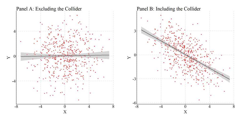
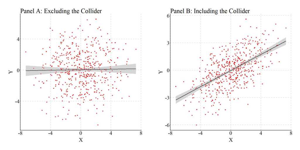
Now let’s estimate the bivariate association between X and Y, as well as the association between X and Y after adjusting for C (i.e., the collider). Just to make sure you believe me, I want to provide you with the results as both syntax and figures. As demonstrated in the first model – Y regressed on X – slope coefficient of b = .016 (p = .706) provides evidence suggesting that Y and X are unrelated (illustrated in Panel A of the figure below). This result is consistent with the specification of the data were variation in X was not specified to cause variation in Y (or vice versa). Nevertheless, when Y is regressed on X and C – the second model – the estimated slope coefficient suggests that X does cause variation in Y. Specifically, a 1-point increase (or decrease) in X appears to be associated with a .816 decrease (or increase) in Y. The observed negative association is statistically significant at the p < .001 level and the visual illustration (Panel B) suggests that a strong association between X and Y exists.
> summary(lm(y~x))

Call:
lm(formula = y ~ x)

Residuals:
         Min           1Q       Median           3Q          Max
-7.139868316 -1.667583254  0.038898907  1.769745904  6.482678410

Coefficients:
                Estimate   Std. Error t value Pr(>|t|)
(Intercept) 0.0472380429 0.1122933055 0.42067  0.67418
x           0.0164779548 0.0436787351 0.37725  0.70615

Residual standard error: 2.50941291 on 498 degrees of freedom
Multiple R-squared:  0.000285701863,	Adjusted R-squared:  -0.00172175657
F-statistic: 0.142320189 on 1 and 498 DF,  p-value: 0.70614595

> summary(lm(y~x+c))

Call:
lm(formula = y ~ x + c)

Residuals:
         Min           1Q       Median           3Q          Max
-3.529044556 -0.769445860  0.021351340  0.739786582  3.216551591

Coefficients:
                 Estimate    Std. Error   t value             Pr(>|t|)
(Intercept)  0.0101428998  0.0507314166   0.19993              0.84161
x           -0.8164554579  0.0273172709 -29.88789 < 0.0000000000000002 ***
c            0.4088164989  0.0092730205  44.08666 < 0.0000000000000002 ***
---
Signif. codes:  0 ‘***’ 0.001 ‘**’ 0.01 ‘*’ 0.05 ‘.’ 0.1 ‘ ’ 1

Residual standard error: 1.1335365 on 497 degrees of freedom
Multiple R-squared:  0.79642253,	Adjusted R-squared:  0.795603305
F-statistic: 972.165527 on 2 and 497 DF,  p-value: < 0.0000000000000002220446

>
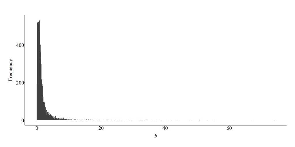
To further demonstrate the bias generated from the inclusion of a collider in a multivariable regression model, we can specify a looped simulation analysis. For the looped simulation analysis, we told the computer to conduct 10,000 simulations (n), where the slope coefficient of the association between X and C, and Y and C, randomly varied between 1 and 100 on a uniform distribution. Moreover, the number of cases in the simulation were randomly selected between 100 and 1000 (on a uniform distribution), and the distribution of X, Y, and C were randomly specified to have a mean between -5 and 5 on a uniform distribution and a standard deviation between 1 and 5 on a uniform distribution. After simulating the data, a regression model was estimated where the slope coefficient of the association between X and Y was adjusted for the influence of C. The estimated slope coefficient was than recorded and used to generate the plot below.
n<-10000

DATA1 = foreach (i=1:n, .packages='lm.beta', .combine=rbind) %dopar%
  {
    N<-sample(100:1000, 1)
    x<-runif(1,1,100)*rnorm(N,runif(1,-5,5),runif(1,1,5))
    y<-runif(1,1,100)*rnorm(N,runif(1,-5,5),runif(1,1,5))
    c<-runif(1,1,100)*x+runif(1,1,100)*y+runif(1,1,100)*rnorm(N,runif(1,-5,5),runif(1,1,5))
    Data<-data.frame(c,x,y)

    M<-lm(y~x+c, data = Data)
    bXY<-M$coefficients[2]

    data.frame(i,bXY)

  }
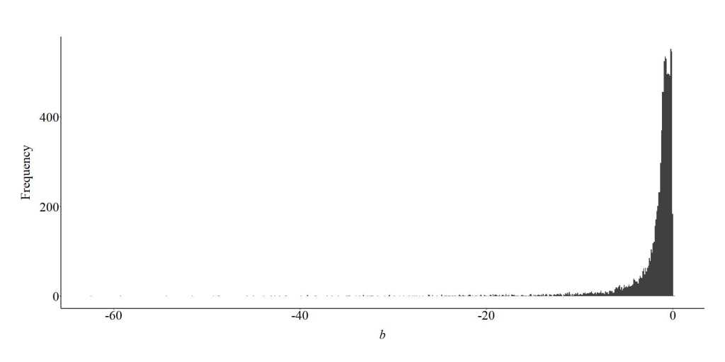
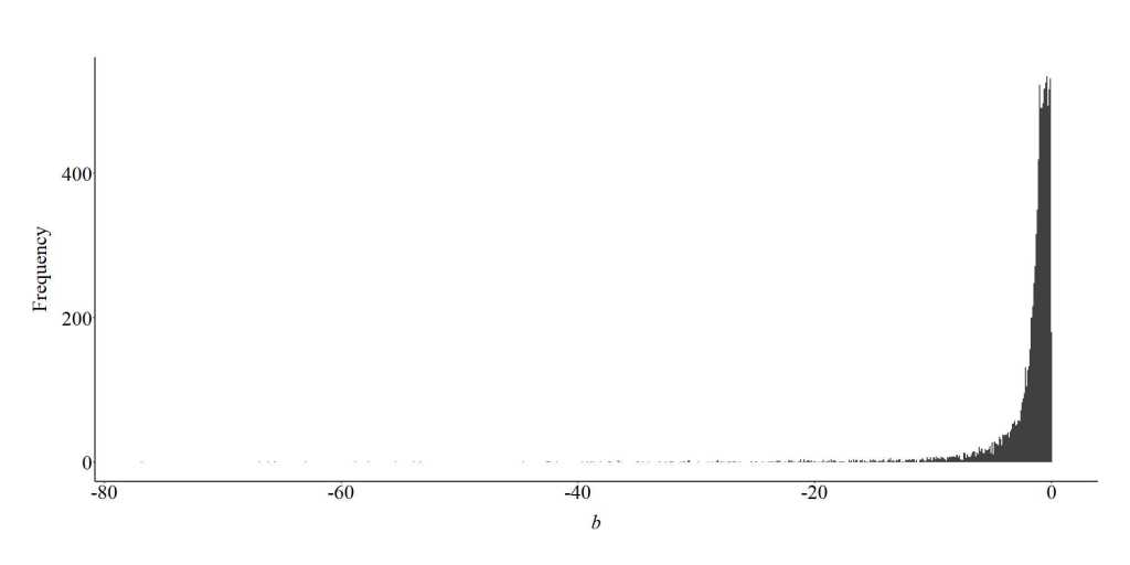
As demonstrated in the plot below, adjusting for a collider (C) between X and Y when estimating the bivariate effects of X on Y will commonly be upwardly (further from zero than reality) biased and regularly generate a negative slope coefficient. The magnitude of the bias, as demonstrated by the illustration, depends upon the magnitude of the collision between X and Y on C. This finding suggests that adjusting for a collider in a multivariable model increases our likelihood of committing a type 1 error (i.e., reject the null hypothesis when in reality the null hypothesis should have been retained).
Collider (-,+)
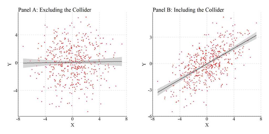
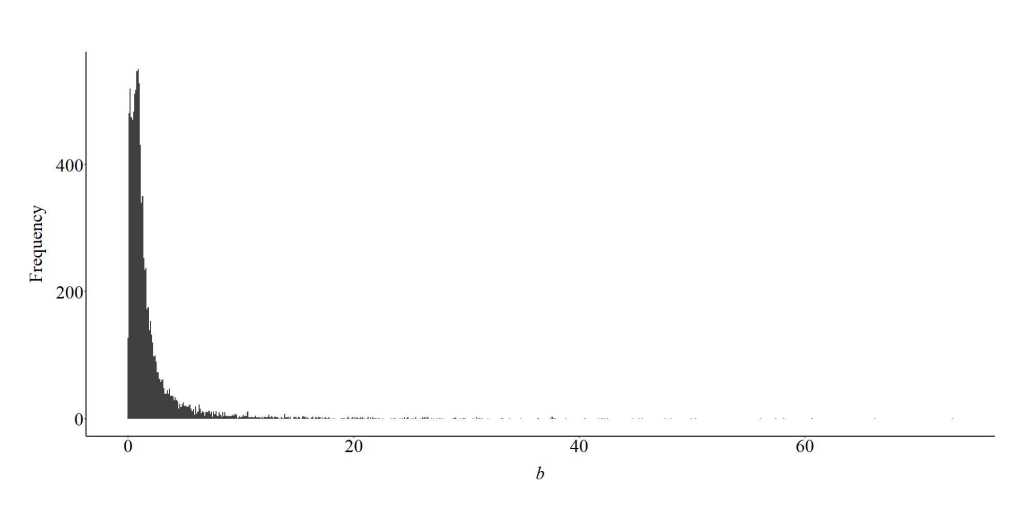
As stated before, however, the direction (i.e., positive or negative association) of the causal influence of X on C, and Y on C, dictates the direction of the bias generated when we condition the slope coefficient of the association between X and Y on C. To illustrate this, we replicated the above simulation, except specified that X was negatively associated with C, where a 1-point increase (or decrease) in X caused a 2-point decrease (or increase) in C. The findings, provided in the figure below, demonstrated that when X and Y have opposite causal effects on C, the slope of the association between X and Y after adjusting for C becomes upwardly biased and positive. Specifically, a 1-point increase in X was associated with a .819 increase in Y (p < .001).
To replicate the looped simulation, we permitted the computer to randomly select any value between -100 and -1 on a uniform distribution to serve as the slope coefficient for the causal influence of X on C. The remainder of the looped simulation was identical to the looped simulation syntax provided above. Consistent with the findings presented by the non-looped simulation analysis, the looped simulation suggested that the slope coefficient of the association between X and Y will commonly become upwardly biased (further from zero than reality) and positive when a collider (C) is adjusted for in a multivariable model. Moreover, similar to the previous specification, we possess an increased likelihood of committing a Type 1 error when a model estimating the effects of an independent variable on a dependent variable is conditioned upon a collider.

Collider (+,-)
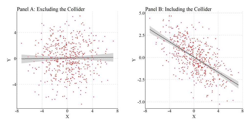
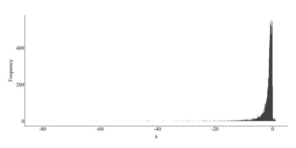
To observe if the opposite specification produced similar findings, we replicated the simulation again. This time, we specified that the association between Y and C was negative, where a 1-point increase (or decrease) in Y was associated with a 2-point decrease (or increase) in C. The remainder of the simulation was identical to the previous examples. The findings further supported the previous demonstration, suggesting that when X and Y have opposite causal effects on C, the slope of the association between X and Y conditioned upon the collider becomes upwardly biased and positive. In this case, the slope coefficient was close to the previous example and suggested that a 1-point increase in X was associated with a .797 increase in Y (p < .001).
Moreover, the looped simulations again demonstrated that the slope coefficient of the association between X and Y will commonly become upwardly biased (further from zero than reality) and positive when the association between X and Y is estimated after adjusting for the effects of the collider (C) in a multivariable model. The specification for the looped simulations permitted the computer to randomly select any value between -100 and -1 on a uniform distribution to serve as the slope coefficient for the causal influence of Y on C, while the slope coefficient of the causal influence of X on C was randomly selected by the computer on a uniform distribution between 1 and 100.
Collider (-,-)
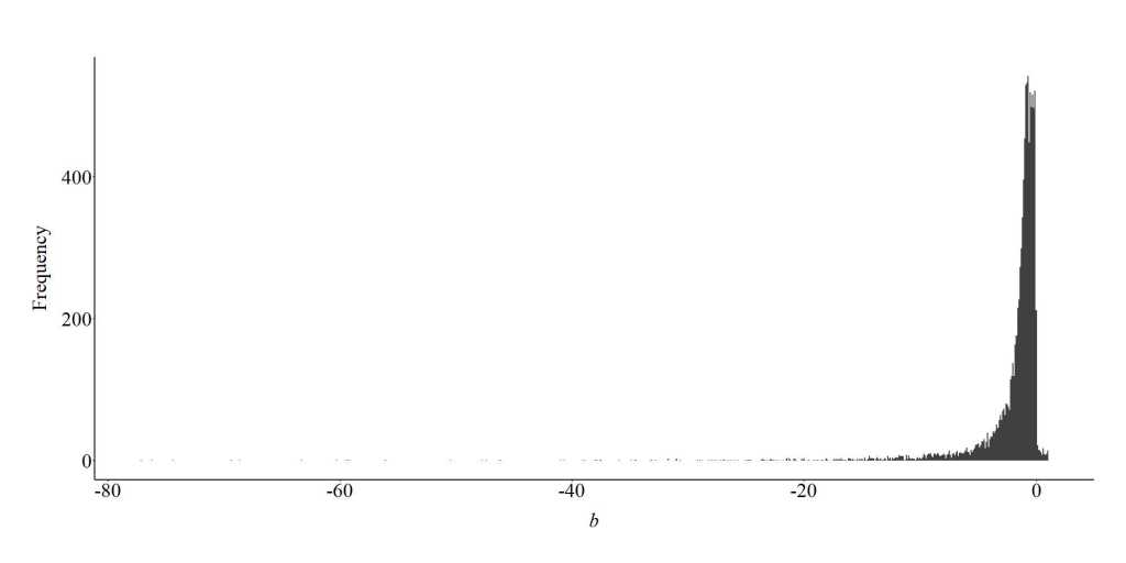
For the final simulation – where the true slope coefficient of the association between X and Y equaled 0 – we replicated the first simulation, but specified that both X and Y had a negative causal influence on the collider (C). Specifically, a 1-point increase (or decrease) in X or Y was specified to cause a 2-point decrease (or increase) in the collider. After simulating the data using code similar to the code above, we estimated the slope coefficient of the association between X and Y with and without adjusting for the influence of the collider (C). Similar to the findings of the first simulation, the slope coefficient of the association between X and Y adjusted for the influence of the collider (C) was upwardly biased (further from zero than reality) and a negative value. Specifically, the results suggested that a 1-point increase (or decrease) in X predicted a .787 decrease (or increase) in Y.
The looped simulations supported these findings, indicating that when X and Y have a negative collision on C, the slope of the association between X and Y adjusted for C commonly becomes negative and further from zero.
Intermission Discussion
As demonstrated above, the inclusion of a collider when estimating an association between an independent and dependent variable will commonly upwardly bias (further from zero than reality) the slope coefficient if the true slope coefficient is zero.[i] The direction – positive or negative values – of that bias, however, varies depending upon the direction of the effects of the independent and dependent variables on the collider. If the effects are in the same direction (e.g., the independent and dependent variables both positively [or negatively] influence variation in the collider) the upward bias will generally be in the negative direction. If the effects are in different directions (e.g., the independent variable positively [or negatively] influences variation in the collider, while the dependent variable negatively [or positively] influences variation in the collider) the upward bias will generally be in the positive direction.
To briefly discuss, the inclusion of a collider biases the slope coefficient – and other estimates – of the association between the independent and dependent variable because the remaining variation in the model after stratification is just the variation in the collider facing the opposite direction. Explicitly, multivariable regression models remove all of the shared variation in the collider – the variation caused by the independent and dependent variables. Nevertheless, the variation that remains after adjusting for the collider is just the shared variation in the opposite direction. This is because the unadjusted for variation in the collider is still common variation between the independent and dependent variables. The shared variation being in the opposite direction is the reason that the slope coefficient between the independent variable and dependent variable is the opposite direction of the collision (e.g., X and Y are positively associated with the collider, but negatively associated with each other when a multivariable model adjusts for said collider). I know this was not a relaxing intermission, but let’s continue with our regularly scheduled program.
True Association Between X and Y = 1
Similar to confounder bias, collider bias can generate Type 2 errors and interpretations in the opposite direction when the true slope coefficient of the association between the independent variable and dependent variable is not equal to zero (Type S error). To evaluate the likelihood of committing a Type 2 error or an interpretation in the incorrect direction, the four looped simulations discussed above were replicated except now the association between X and Y was specified to be equal to 1.00.
Collider (+,+)
As demonstrated in the figure below, when the association between X and Y is conditioned on a collider, where both the independent variable and the dependent variable positively influence variation in the collider, the estimated slope coefficient will generally be lower than the true slope coefficient (b = 1). Under these circumstances, we have a higher likelihood of committing a Type 2 error – retaining the null hypothesis when it should have been rejected – or perceiving that the independent variable (X) has a negative influence on the dependent variable (Y). Overall, this finding indicates that collider bias can both downwardly (closer to zero than the true association) or upwardly bias (further from zero than the true association) the estimated slope coefficient in the wrong direction when the association between X and Y is conditioned upon the variation in a collider.
Collider (-,+)
Similar to the previous replication, the current simulation specified that the collider was differentially influenced by the independent and dependent variables. Specifically, increased scores on X were specified to be associated with decreased scores on the collider, while increased scores on Y were specified to be associated with increased scores on the collider. Evident by the findings, it appears that the model conditioned upon the collider will generally produce a slope coefficient that is larger than the true slope coefficient (b = 1.00). However, on some occasions the slope coefficient can be closer to zero than the true slope coefficient (b = 1.00).

Collider (+,-)
Conditioning upon a collider where the independent variable is positively associated with the collider, but the dependent variable is negatively associated with the collider appeared to commonly upwardly bias the estimated slope coefficient. That is, the estimated slope coefficient was generally further from zero than the true slope coefficient (b = 1.00). Nevertheless, on some occasions the estimated association between X and Y was closer to zero than the true slope coefficient (b = 1.00). The estimated slope coefficient always appeared to be a positive value, but conditioning upon a differentially influenced collider – where X and Y cause variation in opposite directions – can generate both Type 1 and Type 2 errors.
Collider (-,-)
Finally, when both the independent variable and dependent variable negatively influence variation in the collider, conditioning a model upon the collider will generally produce a slope coefficient smaller than the true slope coefficient. Similar to the first simulation, this generates an increased likelihood of committing a Type 2 error – retaining the null hypothesis when it should have been rejected – or perceiving that the independent variable (X) has a negative influence on the dependent variable (Y).
Conclusion
As demonstrated throughout Entry 8, accidentally conditioning an association of interest upon a collider – a variable causally influenced by both the independent and dependent variable – can introduce bias into the statistical estimates generated from our models. The estimated slope coefficients can be upwardly biased (further from zero than the true slope coefficient) or downwardly biased (closer to zero than the true slope coefficient) and in the same direction (e.g., positive true b and positive estimated b) or opposite direction (e.g., positive true b, but negative estimated b) conditional upon the interrelationship between the variables. Considering this, scholars should always express caution when selecting variables to include in multivariable statistical models. The likelihood of accidentally including a collider between an independent variable and the dependent variable in a multivariable regression model is substantively higher than we perceive.
[i] I have now implemented caution in my statements, because there are some anomalies that appear to be bugs in the simulations. Specifically, some data specifications in the looped simulations appear to produce slope coefficients on zero. These bugs could exist for a variety of reasons and, unfortunately, I have not had the opportunity to explore why or how these bugs exist. In theory though, collider bias – similar to confounder bias – can only serve to upwardly bias estimates if the true causal association is 0.
License: Creative Commons Attribution 4.0 International (CC By 4.0)

3 thoughts on “Entry 8: The Inclusion of Colliders (Collider Bias)”