As introduced in Entry 5, the random assignment of respondents to a treatment or a control is fundamental to the process of conducting a true experiment. We assume that random assignment will remove the possibility of an unknown variable confounding the association between exposure to the treatment and an outcome of interest. Under this assumption, random assignment permits the ability to make causal inferences about the effects of the treatment. This assumption, however, does not provide us with the ability to direct observe the causal effects of a treatment (the variation in the outcome directly caused by the treatment). Specifically, covariate balance across the treatment and control cases is needed to observe the causal effects of a treatment. In the current context, covariates refer to any observable or unobservable construct that can influence the outcome of interest. Covariate balance oftentimes is not achieved within a single randomized controlled trial. Only when enough replications of the randomized controlled trial are conducted can we assume – through reliance on central limit theorem – that covariate balance between the treatment and control cases is established. As illustrated throughout the current entry, when covariate balance is not achieved – violations of the assumption of covariate balance –the treatment effects estimated from a single true experiment can deviate substantively from the true causal effects of the treatment in the population.
The Counterfactual
Although it can be described in a variety of manners, a counterfactual can be considered the “what if?” statement to an experiment. Imagine we are conducting a basic experiment in a lab. For simplicity, we are interested in observing what happens when rubbing alcohol is exposed to a flame. We distribute rubbing alcohol from the same bottle evenly into two cups, light a match, and place the match close to the rubbing alcohol in one of the cups. The rubbing alcohol lit on fire. Nevertheless, we can not determine if the match caused the rubbing alcohol to light on fire without observing what happened to the rubbing alcohol in the other cup. As such, we turn to the other cup and observe what happened when the rubbing alcohol is not exposed to the flame. The rubbing alcohol did not appear to light on fire without being exposed to the flame. Considering everything else is equal, we can determine that exposing rubbing alcohol to a flame caused it to light on fire.
As alluded to throughout the example, a true counterfactual condition can only be established when all of the characteristics of the experiment are replicated except for the treatment being varied (e.g., flame vs. no flame). Due to this requirement, a true counterfactual can not be established when conducting an experiment with humans because the participants exposed to the treatment and the participants exposed to the control will differ. These differences could arise for a host of reasons, including sociological differences, biological differences, different life-course histories, etc. Moreover, differences on these key characteristics are likely to influence our outcome of interest, generating a need to establish covariate balance.
The Assumption of Covariate Balance
Our best opportunity to approximate a true counterfactual condition when conducting an experiment with humans is through the establishment of covariate balance. Covariate balance in the context of a counterfactual refers to the condition where cases assigned to the treatment group vary identically to cases assigned to the control group across all key characteristics. To provide an example, our treatment and control groups will be balanced on age if the mean, standard deviation, skewness, and kurtosis of the distribution is identical across the two groups. Any differences, however, will be indicative of covariate imbalance (i.e., the characteristics of the participants are not equal across the treatment and control groups).
When conducting a true experiment, we randomly assign participants to the treatment and control groups under the assumption that (1) variation in the treatment will not be predicted by a confounding variable and (2) covariate balance will be established. Satisfying the first assumption permits causal inferences to be made, while satisfying the second assumption permits the identification of the true effect size of the treatment in the population (i.e., the causal effects of a treatment in the population).[i] Random assignment for a single experiment, however, commonly does not satisfy the second assumption. Specifically, simply randomly assigning participants increases the likelihood of covariate imbalance across the treatment and control groups in a single experiment. Nevertheless, while the assumption of covariate balance is commonly violated in a single experiment, multiple replications using random assignment will ensure that the second assumption is satisfied when a meta-analysis is conducted.
Violations of The Assumption of Covariate Balance
Let’s begin the illustration by simulating the treatment population and the control population separately. By simulating the treatment and control populations separately, we can ensure that the specified covariates are identical – balanced – across the two populations. First, let us begin with the treatment population. The specification below simulates 50,000 cases with a value of 1 on the treatment (“Tr” in the R-code) variable. In addition to the treatment variable, four additional variables are simulated for the treatment cases. These include a dichotomous variable (“DI1” in the R-code), a categorical variable (“DV1” in the R-code), a semi-continuous variable (“SCV1” in the R-code), and a continuous variable (“CV1” in the R-code). After which, we merge all of the measures into a single dataframe. Importantly, the seed for the simulation was set to 1992 to ensure the process can be replicated.
## Treatment Cases ####
set.seed(1992)
N<-50000
Tr<-rep(1,N)
DI1<-rep(c(0,1),length.out = N) # Dichotomous Variable
DV1<-trunc(rnorm(N,2.5,.75)) # Categorical Variable
SCV1<-trunc(rnorm(N,35,5)) # Semi-continuous Variable
CV1<-trunc(rnorm(N,35000,5000)) # Continuous Variable

Treat.DF<-data.frame(Tr,DI1,DV1,SCV1,CV1)
After simulating the treatment population, the simulation is replicated for the control population except for scores on the treatment variable being equal to “0” instead of “1” (“Tr” in the R-code).
## Control Cases ####
set.seed(1992)
N<-50000
Tr<-rep(0,N)
DI1<-rep(c(0,1),length.out = N) # Dichotomous Variable
DV1<-trunc(rnorm(N,2.5,.75)) # Categorical Variable
SCV1<-trunc(rnorm(N,35,5)) # Semi-continuous Variable
CV1<-trunc(rnorm(N,35000,5000)) # Continuous Variable

Control.DF<-data.frame(Tr,DI1,DV1,SCV1,CV1)
As a brief check, let’s make sure that the mean, standard deviation, skew, and kurtosis for the four additional variables (i.e., DI1; DV1; SCV1; CV1) are identical between the treatment and control populations. This check is conducted by subtracting the mean for the control group from the mean of the treatment group, the standard deviation for the control group from the standard deviation of the treatment group, and so on. The zeros across the board indicate that the treatment and control populations are identical.
> mean(Treat.DF$DI1)-mean(Control.DF$DI1)
[1] 0
> sd(Treat.DF$DI1)-sd(Control.DF$DI1)
[1] 0
> skew(Treat.DF$DI1)-skew(Control.DF$DI1)
[1] 0
> kurtosi(Treat.DF$DI1)-kurtosi(Control.DF$DI1)
[1] 0
>
> mean(Treat.DF$DV1)-mean(Control.DF$DV1)
[1] 0
> sd(Treat.DF$DV1)-sd(Control.DF$DV1)
[1] 0
> skew(Treat.DF$DV1)-skew(Control.DF$DV1)
[1] 0
> kurtosi(Treat.DF$DV1)-kurtosi(Control.DF$DV1)
[1] 0
>
> mean(Treat.DF$SCV1)-mean(Control.DF$SCV1)
[1] 0
> sd(Treat.DF$SCV1)-sd(Control.DF$SCV1)
[1] 0
> skew(Treat.DF$SCV1)-skew(Control.DF$SCV1)
[1] 0
> kurtosi(Treat.DF$SCV1)-kurtosi(Control.DF$SCV1)
[1] 0
>
> mean(Treat.DF$CV1)-mean(Control.DF$CV1)
[1] 0
> sd(Treat.DF$CV1)-sd(Control.DF$CV1)
[1] 0
> skew(Treat.DF$CV1)-skew(Control.DF$CV1)
[1] 0
> kurtosi(Treat.DF$CV1)-kurtosi(Control.DF$CV1)
[1] 0
>
Now that we have identical treatment and control populations, we can merge the dataframes – creating the overall population – and specify that scores on the dependent variable (“Y”) were equal to 10 times the treatment, 1.25 times DI1, .25 times DV1, .0075 times SCV1, and .0075 times CV1.[ii]
## Creating Population ####


Pop<-rbind(Treat.DF,Control.DF)

table(Pop$Tr)

## Creating Outcome Variable ####

names(Pop)

Pop$Y<-(10.00*Pop$Tr)+(1.25)*Pop$DI1+(.25*Pop$DV1)+(.0075*Pop$SCV1)+(.0075*Pop$CV1)
summary(Pop$Y)
Now that we have created our simulated dataset, let’s run some randomized controlled trials. As a reminder, it takes some mental gymnastics to work through simulated randomized controlled trials. Specifically, it is difficult to simulate a randomized controlled trial because scores on the treatment variable are not influenced by any other construct. As such, we are unable to reassign exposure to the treatment variable when samples are pulled from the population. For each sample we pull, just imagine that a randomized controlled trial is being conducted.
Randomized Controlled Trial 1: Sample of 100
To conduct our first randomized controlled trial, we sampled 50 treatment cases and 50 control cases from the population. The seed for this sampling procedure was set specified as 633487.[iii] After randomly sampling treatment and control cases from the population, we need to evaluate if the covariates are balanced across the treatment and control cases. As a reminder, for us to define the covariates as balanced the characteristics of the participants must be equal across the two groups. While definitions of equal vary, this is generally defined as non-significant differences between the two groups. Personally, I don’t like to define distributional differences based on p-values, so for this case we will define balance as the evidence generally – I use this term loosely – suggests that there are no distributional differences on the four covariates between the treatment and control cases. Specifically, the differences between the mean, standard deviation, skew, and kurtosis would have to be negligible after considering the range of scores on the covariate.
Considering the results of all of the distributional comparisons between our treatment and control cases, our random selection of cases from the population did not achieve covariate balance, violating the assumption of covariate balance. Specifically, the distributional differences appeared minimal for the dichotomous and categorical variable, but more substantive for the semi-continuous and continuous variables. By violating the assumption of covariate balance, we have unfortunately biased the estimates derived from our randomized controlled trial. In this case, the estimated effect of the treatment on the dependent variable (Y) was 18.93, which is almost double the true effect size of the treatment in the population (10.00). These results illustrate the importance of satisfying the covariate balance assumption when conducting a true experiment.
> # 1 Sample (N = 100) ####
> set.seed(633487)
> TMC<-sample_n(Pop[which(Pop$Tr == 1),] ,50, replace = F)
> CMC<-sample_n(Pop[which(Pop$Tr == 0),] ,50, replace = F)
>
> # Dichotomous Variable
> mean(TMC$DI1)-mean(CMC$DI1)
[1] -0.06
> sd(TMC$DI1)-sd(CMC$DI1)
[1] 0.001215
> skew(TMC$DI1)-skew(CMC$DI1)
[1] 0.2334
> kurtosi(TMC$DI1)-kurtosi(CMC$DI1)
[1] -0.01859
>
> # Categorical Variable
> mean(TMC$DV1)-mean(CMC$DV1)
[1] 0.24
> sd(TMC$DV1)-sd(CMC$DV1)
[1] -0.0829
> skew(TMC$DV1)-skew(CMC$DV1)
[1] -0.4097
> kurtosi(TMC$DV1)-kurtosi(CMC$DV1)
[1] 0.8232
>
> # Semi-continuous Variable
> mean(TMC$SCV1)-mean(CMC$SCV1)
[1] -1.14
> sd(TMC$SCV1)-sd(CMC$SCV1)
[1] 0.8317
> skew(TMC$SCV1)-skew(CMC$SCV1)
[1] -0.2257
> kurtosi(TMC$SCV1)-kurtosi(CMC$SCV1)
[1] 0.1349
>
> # Continuous Variable
> mean(TMC$CV1)-mean(CMC$CV1)
[1] 1193
> sd(TMC$CV1)-sd(CMC$CV1)
[1] -701.5
> skew(TMC$CV1)-skew(CMC$CV1)
[1] -0.869
> kurtosi(TMC$CV1)-kurtosi(CMC$CV1)
[1] -1.204
>
> DF<-rbind(TMC,CMC)
>
> LM_NRS<-lm(Y~Tr, data = DF)
> summary(LM_NRS)

Call:
lm(formula = Y ~ Tr, data = DF)

Residuals:
   Min     1Q Median     3Q    Max
-86.36 -23.48  -6.25  24.51 129.68

Coefficients:
            Estimate Std. Error t value            Pr(>|t|)
(Intercept)   254.96       5.24   48.69 <0.0000000000000002 ***
Tr             18.93       7.41    2.56               0.012 *
---
Signif. codes:  0 ‘***’ 0.001 ‘**’ 0.01 ‘*’ 0.05 ‘.’ 0.1 ‘ ’ 1

Residual standard error: 37 on 98 degrees of freedom
Multiple R-squared:  0.0625,	Adjusted R-squared:  0.0529
F-statistic: 6.53 on 1 and 98 DF,  p-value: 0.0121

>
One question that remains: does the sample size of the treatment and the control groups in a randomized controlled trial matter for satisfying the assumption of covariate balance? As demonstrated by the three replications of the first simulation with varying sample sizes (N = 200; N = 500; N = 1000), it does.
Randomized Controlled Trial 2: Sample of 200
>
> set.seed(267714)
> TMC<-sample_n(Pop[which(Pop$Tr == 1),] ,100, replace = F)
> CMC<-sample_n(Pop[which(Pop$Tr == 0),] ,100, replace = F)
>
>
> # Dichotomous Variable
> mean(TMC$DI1)-mean(CMC$DI1)
[1] -0.03
> sd(TMC$DI1)-sd(CMC$DI1)
[1] -0.0003017
> skew(TMC$DI1)-skew(CMC$DI1)
[1] 0.1183
> kurtosi(TMC$DI1)-kurtosi(CMC$DI1)
[1] 0.004714
>
> # Categorical Variable
> mean(TMC$DV1)-mean(CMC$DV1)
[1] -0.01
> sd(TMC$DV1)-sd(CMC$DV1)
[1] 0.07611
> skew(TMC$DV1)-skew(CMC$DV1)
[1] -0.1198
> kurtosi(TMC$DV1)-kurtosi(CMC$DV1)
[1] 0.6161
>
> # Semi-continuous Variable
> mean(TMC$SCV1)-mean(CMC$SCV1)
[1] -0.15
> sd(TMC$SCV1)-sd(CMC$SCV1)
[1] -0.3808
> skew(TMC$SCV1)-skew(CMC$SCV1)
[1] -0.1472
> kurtosi(TMC$SCV1)-kurtosi(CMC$SCV1)
[1] 0.4915
>
> # Continuous Variable
> mean(TMC$CV1)-mean(CMC$CV1)
[1] 1212
> sd(TMC$CV1)-sd(CMC$CV1)
[1] 128.8
> skew(TMC$CV1)-skew(CMC$CV1)
[1] 0.2267
> kurtosi(TMC$CV1)-kurtosi(CMC$CV1)
[1] -0.1588
>
> DF<-rbind(TMC,CMC)
>
> LM_NRS<-lm(Y~Tr, data = DF)
> summary(LM_NRS)

Call:
lm(formula = Y ~ Tr, data = DF)

Residuals:
   Min     1Q Median     3Q    Max
-84.28 -21.64   0.95  21.63 100.18

Coefficients:
            Estimate Std. Error t value             Pr(>|t|)
(Intercept)   258.48       3.52   73.49 < 0.0000000000000002 ***
Tr             19.05       4.97    3.83              0.00017 ***
---
Signif. codes:  0 ‘***’ 0.001 ‘**’ 0.01 ‘*’ 0.05 ‘.’ 0.1 ‘ ’ 1

Residual standard error: 35.2 on 198 degrees of freedom
Multiple R-squared:  0.069,	Adjusted R-squared:  0.0643
F-statistic: 14.7 on 1 and 198 DF,  p-value: 0.000172

>
Randomized Controlled Trial 3: Sample of 500
>
> set.seed(92021)
>
> TMC<-sample_n(Pop[which(Pop$Tr == 1),] ,250, replace = F)
> CMC<-sample_n(Pop[which(Pop$Tr == 0),] ,250, replace = F)
>
>
> # Dichotomous Variable
> mean(TMC$DI1)-mean(CMC$DI1)
[1] 0.028
> sd(TMC$DI1)-sd(CMC$DI1)
[1] 0.0005615
> skew(TMC$DI1)-skew(CMC$DI1)
[1] -0.1114
> kurtosi(TMC$DI1)-kurtosi(CMC$DI1)
[1] -0.00891
>
> # Categorical Variable
> mean(TMC$DV1)-mean(CMC$DV1)
[1] -0.064
> sd(TMC$DV1)-sd(CMC$DV1)
[1] 0.09333
> skew(TMC$DV1)-skew(CMC$DV1)
[1] 0.08768
> kurtosi(TMC$DV1)-kurtosi(CMC$DV1)
[1] -0.5585
>
> # Semi-continuous Variable
> mean(TMC$SCV1)-mean(CMC$SCV1)
[1] 0.032
> sd(TMC$SCV1)-sd(CMC$SCV1)
[1] -0.1224
> skew(TMC$SCV1)-skew(CMC$SCV1)
[1] -0.07692
> kurtosi(TMC$SCV1)-kurtosi(CMC$SCV1)
[1] -0.6315
>
> # Continuous Variable
> mean(TMC$CV1)-mean(CMC$CV1)
[1] 879.8
> sd(TMC$CV1)-sd(CMC$CV1)
[1] -459.2
> skew(TMC$CV1)-skew(CMC$CV1)
[1] 0.2811
> kurtosi(TMC$CV1)-kurtosi(CMC$CV1)
[1] 0.2042
>
> DF<-rbind(TMC,CMC)
>
> LM_NRS<-lm(Y~Tr, data = DF)
> summary(LM_NRS)

Call:
lm(formula = Y ~ Tr, data = DF)

Residuals:
    Min      1Q  Median      3Q     Max
-130.17  -22.38    0.95   23.50  149.28

Coefficients:
            Estimate Std. Error t value             Pr(>|t|)
(Intercept)   257.98       2.26   114.2 < 0.0000000000000002 ***
Tr             16.62       3.19     5.2           0.00000029 ***
---
Signif. codes:  0 ‘***’ 0.001 ‘**’ 0.01 ‘*’ 0.05 ‘.’ 0.1 ‘ ’ 1

Residual standard error: 35.7 on 498 degrees of freedom
Multiple R-squared:  0.0516,	Adjusted R-squared:  0.0496
F-statistic: 27.1 on 1 and 498 DF,  p-value: 0.000000287

>
Randomized Controlled Trial 4: Sample of 1000
> set.seed(21873)
>
> TMC<-sample_n(Pop[which(Pop$Tr == 1),] ,500, replace = F)
> CMC<-sample_n(Pop[which(Pop$Tr == 0),] ,500, replace = F)
>
>
> # Dichotomous Variable
> mean(TMC$DI1)-mean(CMC$DI1)
[1] -0.056
> sd(TMC$DI1)-sd(CMC$DI1)
[1] 0
> skew(TMC$DI1)-skew(CMC$DI1)
[1] 0.2237
> kurtosi(TMC$DI1)-kurtosi(CMC$DI1)
[1] 0
>
> # Categorical Variable
> mean(TMC$DV1)-mean(CMC$DV1)
[1] 0.046
> sd(TMC$DV1)-sd(CMC$DV1)
[1] -0.02973
> skew(TMC$DV1)-skew(CMC$DV1)
[1] -0.1608
> kurtosi(TMC$DV1)-kurtosi(CMC$DV1)
[1] 0.149
>
> # Semi-continuous Variable
> mean(TMC$SCV1)-mean(CMC$SCV1)
[1] 0.276
> sd(TMC$SCV1)-sd(CMC$SCV1)
[1] 0.07067
> skew(TMC$SCV1)-skew(CMC$SCV1)
[1] 0.06591
> kurtosi(TMC$SCV1)-kurtosi(CMC$SCV1)
[1] -0.159
>
> # Continuous Variable
> mean(TMC$CV1)-mean(CMC$CV1)
[1] -345.6
> sd(TMC$CV1)-sd(CMC$CV1)
[1] -144
> skew(TMC$CV1)-skew(CMC$CV1)
[1] 0.2711
> kurtosi(TMC$CV1)-kurtosi(CMC$CV1)
[1] 0.3549
>
> DF<-rbind(TMC,CMC)
>
> LM_NRS<-lm(Y~Tr, data = DF)
> summary(LM_NRS)

Call:
lm(formula = Y ~ Tr, data = DF)

Residuals:
    Min      1Q  Median      3Q     Max
-119.25  -25.64   -2.59   25.84  145.00

Coefficients:
            Estimate Std. Error t value            Pr(>|t|)
(Intercept)   265.45       1.66  159.43 <0.0000000000000002 ***
Tr              7.35       2.35    3.12              0.0018 **
---
Signif. codes:  0 ‘***’ 0.001 ‘**’ 0.01 ‘*’ 0.05 ‘.’ 0.1 ‘ ’ 1

Residual standard error: 37.2 on 998 degrees of freedom
Multiple R-squared:  0.00967,	Adjusted R-squared:  0.00868
F-statistic: 9.75 on 1 and 998 DF,  p-value: 0.00185

>
Discussion
As illustrated by the four simulations, randomization does not always satisfy the assumption of covariate balance. In most situations, randomly assigning cases to the treatment and control groups actually generates a condition where we have imbalance – the mean, standard deviation, skewness, and kurtosis of the distribution is different – between our treatment and control cases on known and unknown covariates. Violations of the assumption of covariate balance will bias the observed effectiveness of a treatment, limiting our ability to identify the true effect size of the treatment in the population. Increasing the sample size of the randomized controlled trial is one potential method for satisfying the assumption of covariate balance. Nevertheless, conducting a large randomized controlled trial is quite expensive. There, however, are alternative methods for achieving covariate balance when conducting randomized controlled trials.
One method to increase covariate balance during a randomized controlled trial is blocked randomization (Efird, 2011; Lachin, Matts, and Wei, 1988). Briefly, blocked randomization is the process of stratifying a sample into strata with similar scores on key covariates and randomly assigning participants from each stratum to the treatment and control groups. For example, a sample of 12 individuals could be stratified into two groups based upon biological sex (6 males in strata 1 and 6 females in strata 2). Then 3 individuals from stratum 1 and 3 individuals from stratum 2 can be randomly assigned to the treatment group, while 3 individuals from stratum 1 and 3 individuals from stratum 2 can be randomly assigned to the control group. Blocked randomization requires the observation of key covariates to identify appropriate strata. While blocked randomization can increase covariate balance, replications are fundamental to satisfying the assumption of covariate balance.
Achieving Covariate Balance Through Replications
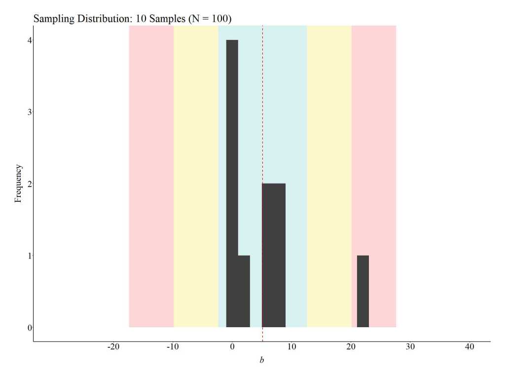
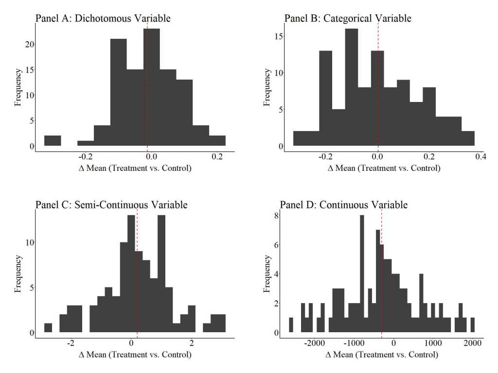
To provide an illustration of how replications can satisfy the assumption of covariate balance, three additional simulations were conducted. For these simulations, we (1) randomly sampled 100 cases (50 treatment cases & 50 control cases), (2) estimated the mean difference between the treatment and control case on the key covariates, (3) estimated the effects of the treatment on the outcome of interest, and (4) repeated the process 10, 100, and 1000 times (respectively).[iv] The results illustrate that the assumption of covariate balance is partially satisfied when a randomized controlled trial is replicated 10 times, but fully satisfied when a randomized controlled trial is replicated 100 or 1000 times. These findings directly illustrate the principles of the central limit theorem and indicate that random assignment can achieve covariate balance if enough replications are conducted. This – in addition to various others – is just another reason why replications are extremely important when conducting experimental research.
10 replications

100 replications

1000 replications
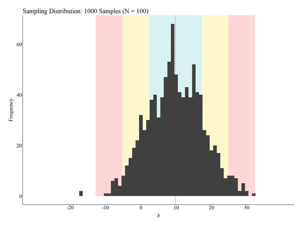
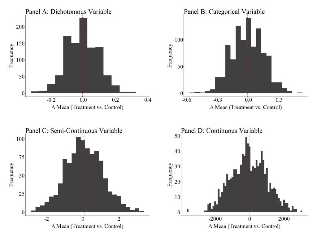
Notes: “Δ mean” is the mean difference between the treatment and control cases on the specified covariate. The red dashed line represents the average of the mean differences across the 1000 replications of the randomized controlled trial (N = 100) on the specified covariate.
Conclusion
As illustrated throughout the current entry, conducting a randomized controlled trial might not satisfy the assumption of covariate balance. Specifically, covariate As illustrated throughout the current entry, conducting a randomized controlled trial might not satisfy the assumption of covariate balance. Specifically, covariate imbalance between the treatment and control cases is likely to exist when participants are simply randomly assigned to the treatment or control conditions. When covariate imbalance exists – a violation of the assumption of covariate balance – the estimated effects of the treatment will likely be biased. While the direction and magnitude of the bias could vary substantively, violations of the assumption of covariate balance hinder our ability to identify the true effect size of the treatment in the population (i.e., the causal effects). Considering the importance of satisfying the assumption of covariate balance, we should (1) proactively employ techniques that increase our ability to satisfy the assumption of covariate balance (e.g., blocked randomization) and (2) replicate randomized controlled trials as frequently as possible.
[i] Importantly, the assumption of covariate balance only matters when variation in the outcome of interest is predicted by known or unknown variation in the population. Considering that almost all outcomes of interest are predicted by known or unknown variation in the population, this assumption must be satisfied to observed the causal effects of a treatment in the population when conducting a true experiment.
[ii] These values were selected based upon the level of measurement for the specified variable, as well as illustrative purposes.
[iii] The seed for these simulations are extremely important, as the seed influences if the randomization procedure generates balance or imbalanced on the covariates across the treatment and control cases. I suggest altering the seed to explore covariate balance when other seed values are used to conduct the random sampling.
[iv] The R-code for this procedure is provided above.
License: Creative Commons Attribution 4.0 International (CC By 4.0)
