Corresponding Publication:
Silver, Ian A. and Kelsay, James D. 2021 “The moderating effects of population characteristics: A potential biasing factor when employing non-random samples to conduct experimental research.” Journal of Experimental Criminology. https://doi.org/10.1007/s11292-021-09478-7.
Conducting a randomized controlled trial is the foremost strategy for estimating a causal association between a treatment variable and an outcome. In the context of a randomized controlled trial, a treatment variable is oftentimes a dichotomous, categorical, or semi-continuous construct that is differentially provided to a sample of participants.[i] For instance, something as common as aspirin can be defined as a treatment variable and provided to participants at different dosages (e.g., 0 pills, 1 pill, 2 pills, etc.). I would note that aspirin is not fully continuous because dosages beyond 10 pills would inevitably result in stomach ulcers. An outcome, or the dependent variable, in a randomized controlled trial is defined as any concept we expect to vary after the introduction of the treatment. To continue with our aspirin example, we would expect to observe differences in back pain after the introduction of aspirin, and the level of pain to vary by the dosage of aspirin.
The most common way of conducting a randomized controlled trial is to randomly select half of the participants to be exposed to a treatment (e.g., the aspirin) and half of the participants to not be exposed to the treatment, otherwise known as the control group (e.g., no aspirin). By randomly assigning participants to the treatment and control groups, we can create a condition where nothing predicts exposure to the treatment. This essentially removes any possibility of an unknown variable confounding the association between exposure to the treatment and an outcome of interest. After randomly assigning participants, we can calculate the difference in the outcome between the treatment cases (i.e., individuals exposed to the treatment) and control cases (i.e., individuals not exposed to the treatment) and evaluate the influence of the treatment on the outcome. The process of conducting a randomized controlled trial, or true experiment, satisfies the three requirements of causality (logical, temporally ordered, and non-spurious) and permits scholars to infer about the causal association between the treatment and the outcome of interest. Moreover, it allows us to assume that the estimates derived from any statistical analysis (e.g., t-test, Anova, OLS regression models) approach causality better than observational studies. Nevertheless, for the estimates derived from a single, or multiple, randomized controlled trials to permit inferences of causal associations in the population two key assumptions must be satisfied: (1) the assumption of known treatment interactions and (2) the assumption of balance between the treatment and control cases.[ii]
A Research Note: The Importance of Replication to Causal Inference
Causal inference through experimental design can not be achieved without replication. A fundamental assumption of experimental research is that the experiment will be conducted multiple times and the findings will be aggregated to create a distribution of findings illuminating the causal effects of the treatment on the outcome. Although the findings of a single randomized controlled trial can be used to make inferences about causal associations, the true causal effects in the population will remain unknown until replications are conducted. As such, replications are key to all research, but are especially important for experimental research. Let this brief note serve as a reminder that more replications need to be conducted. Reminders about the importance of replications will appear throughout the Sources of Statistical Biases Series. Now back to our regularly scheduled program.
The Assumption of Known Interactions
An interaction refers to a condition where the effects of an independent variable on a dependent variable change across levels of a third variable. For example, the magnitude of the effect of GPA on placement in a law firm will vary by the law school an individual attended. In theory, higher GPA would predict better placement, but the magnitude of the effect will change if an individual attended Harvard law or the University of Cincinnati law school (Go Bearcats!). To use statistical terms, the third variable (e.g., the law school attended) moderates the association between the independent variable and the dependent variable. In complex systems, like topics studied in the social sciences, numerous interactions between constructs exist.
When conducting analyses on data collected during randomized controlled trials, we oftentimes either assume that the effects of the treatment on the outcome is not moderated by a third construct or that we know the moderating mechanisms. This is the assumption of known interactions. The assumption of known interactions, however, is difficult to satisfy because it requires the identification of the possible moderators before the randomized controlled trial is conducted. As such, we can never know if we have identified all of the possible constructs that influence the association between the treatment and outcome of interest.
Violating the known interaction assumption does not hinder the ability of randomized controlled trials to estimate causal associations. Violations, however, could substantially hinder our ability to generate causal inferences using data from a randomized controlled trial. More specifically, the estimates from randomized controlled trials that violate the assumption of known interactions could limit the generalizability of the findings, as well as diminish our understanding of the causal association between the treatment and the outcome of interest. Nevertheless, the detrimental effects of unknown interactions only become important when the initial sample is pulled from the broader population using non-random sampling techniques. As illustrated below, only a random sample from the population will produce a sampling distribution that encompasses the causal association in the broader population. Additionally, data from randomized controlled trials employing non-random sampling techniques could produce sampling distributions contrasting with the true effects of the treatment on the outcome.
Simulating the Population
For the purpose of illustrating the effects of unknown interactions, we will conduct a simulated – I know surprising, right? – randomized controlled trial evaluating the effects of a hypothetical employment program on hypothetical success in employment scale. For this example, an interaction between the employment program and parent education will exist in the population. In this simulation, we will specify that the employment program is less effective for individuals with higher parent education and more effective for individuals with lower parent education.
Now that we grasp the example, let me begin the simulation by stating a simple truth; It will take some mental gymnastics to work through this example. Two things in particular are important to remember or more specifically forget. First, even though we build an interaction between the employment program and parent education, we are going to imagine that we don’t know that interaction exists. So, after we build the population forget about that interaction! Second, it is difficult to simulate a randomized controlled trial because scores on the treatment variable are not influenced by any other construct, as well as the need to specify exposure to the treatment variable (i.e., the education program) before we create the outcome (i.e., success in employment). Although not important in the population, when samples are pulled from the population, we are unable to reassign exposure to the treatment variable. As such, we need to imagine that the randomized controlled trial is being conducted in each sample we pull.
For the population, we will randomly assign 500,000 cases to be exposed to the employment program or not exposed to the employment program (250,000 each). After randomly designating cases as treatment or control, the cases were assigned scores on parental education – conceptualized as highest grade completed. The scores were simulated to be normally distributed, with a mean of 12 (representing 12th grade), and a standard deviation of 2.5 grades. Although scores on parental education initially ranged between 0 and 23, we truncated the distribution to range between 4th grade (all scores below 4 received a score of 4) and 19th grade (all scores above 19 received a score of 19). This decision was made to keep the distribution of scores realistic and serves no purpose for the actual illustration.
> ## Building Population (N = 500,000) ####
> ### (X) Example Variable: Employment Program
> set.seed(7)
> EP<-rep(c(0,1),times=250000)
> table(EP)
EP
     0      1
250000 250000
>
> ### (M[moderator]) Example Variable: Parental Educational Attainment
> set.seed(1121)
> PEA<-trunc(rnorm(500000,12,2.5))
> PEA[PEA<=4]<-4 # Making Lowest Grade Completed 4th grade (For example purposes)
> PEA[PEA>=19]<-19 # Making Highest Grade Completed 19th grade (For example purposes)
> table(PEA)
PEA
    4     5     6     7     8     9    10    11    12    13    14    15    16    17
 1295  2904  7122 15874 30260 48594 66516 77422 78113 66457 48261 29883 16004  7200
   18    19
 2759  1336
After simulating exposure to the employment program and parental education, we can create the success in employment construct. The modifying values in the initial specification are uninformative because of the inclusion of an interaction term [(-.50*(PEA*EP))] and the inclusion of some normally distributed variation [rnorm(500000,5,.25)]. As such, we estimate a baseline model to identify the effect of the employment program on success in employment for the population (N = 500,000). The estimated coefficient, b = 1.25, represents the difference on success in employment between the treatment and control cases across the entire population, where the treatment cases will score 1.25 points higher than control cases on success in employment.
> ### (Y) Example Variable: Success In Employment
> ### Higher scores means more success, Lower scores means less success
> set.seed(39817)
> SIEM<-7.00*EP+0.0*PEA+(-.50*(PEA*EP))+rnorm(500000,5,.25)
>
> A<-data.frame(EP,PEA,SIEM)
>
> lm(SIEM~EP, data = A)

Call:
lm(formula = SIEM ~ EP, data = A)

Coefficients:
(Intercept)           EP
       5.00         1.25
For illustrative purposes, let’s take a moment to look at the distribution of scores on success in employment for the treatment (the red distribution) and control groups (the light blue distribution). As you probably noticed, the distribution of success in employment for the treatment group is wider (more platykurtic), while the distribution of success in employment for the control cases is narrower (more leptokurtic). The distributional differences between the two groups is a direct result of: (1) the effects of the employment program, (2) the interaction between the employment program and parental education.
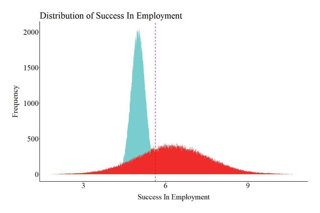
Notes: Red represents the treatment group (individuals exposed to the employment program) and light blue represents the control group (individuals not exposed to the employment program).
Sampling Distribution of Association: Random Sample of Population
For the first illustration, we will randomly sample 1,000 cases from the population and estimate the effects of the employment program on success in employment. However, while one sample can be informative, repeating this process various times could help us develop a sampling distribution of the effects of the employment program on success in employment. As such, using a loop in R, a random sample of 1,000 cases was drawn from the population 10,000 times. Each time a random sample was drawn, our code informed R to estimate and record the slope coefficient and standard error of the association between the employment program and success in employment. This looped simulation simply mirrors how we would conduct randomized controlled trials if money and time were of no concern: (1) randomly sample from the population, (2) randomly expose cases to a treatment or control condition, (3) evaluate differences in the outcome, and (4) replicate the process.
>N<-10000
>RSDF1 <- new.env()
>### Loop
>for(i in 1:N)
>{
>RS1<-sample_n(A, 1000, replace = F)
>
>LM_RS<-lm(SIEM~EP, data = RS1)
>summary(LM_RS)
>
>RSDF1$Slope<-c(RSDF1$Slope, summary(LM_RS)$coefficients[2])
>RSDF1$SE<-c(RSDF1$SE, summary(LM_RS)$coefficients[4])
>}
The distribution of estimated slope coefficients (b) – the sampling distribution – derived from the 10,000 random samples of 1,000 respondents is provided in the figure below. The red dashed line represents the mean slope coefficient, while the blue, yellow, and red areas represent 1, 2, and 3 (respectively) standard deviations from the mean. As illustrated by the figure, the mean of the sampling distribution for the slope coefficient (b = 1.25) – the difference on success in employment between the treatment and control cases – is almost identical to the difference observed for the entire population (b = 1.25). Moreover, only a limited number of random samples drawn from the population were observed to have differences on success in employment between the treatment and control cases (i.e., slope coefficients) smaller than 1.07 and larger than 1.44. Overall, this finding suggests that participation in the employment program will cause an increase of 1.25 on success in employment independent of who receives the program.
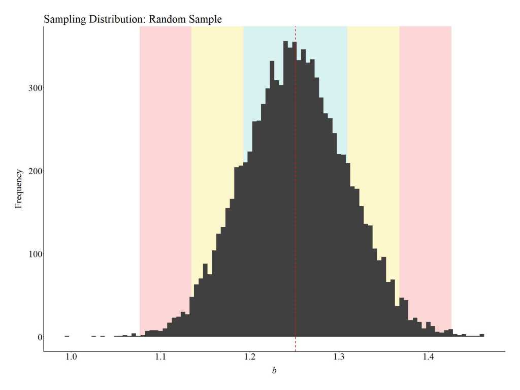
Notes: The red dashed line represents the mean slope coefficient, while the blue, yellow, and red areas represent 1, 2, and 3 (respectively) standard deviations from the mean.
Sampling Distribution of Association: Non-Random Samples of the Population
High Levels Parental Education (PEA>=15)
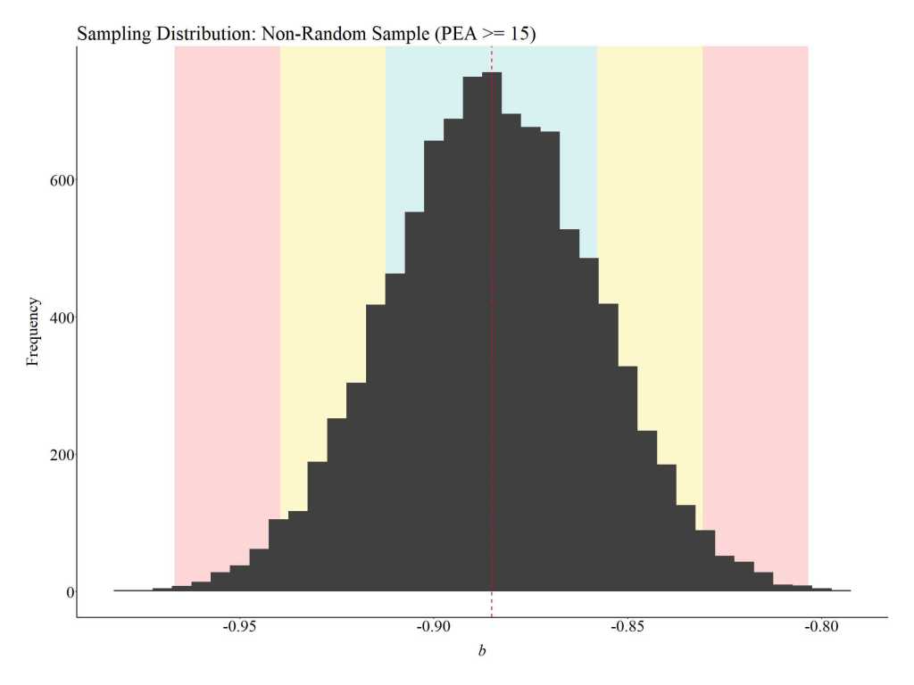
Now let’s repeat the process with a non-random convenience sample.[ii] How about we only sample from individuals with high levels of parental education? When the slope coefficients from the 10,000 non-random samples of 1,000 participants with high parental education are plotted the findings suggest that participation in the employment program causes a -.88 reduction in success in employment. Moreover, the range of the sampling distribution suggests that the employment program will approximately cause between a 1 to .75 reduction in success in employment.
>N<-10000
>RSDF1 <- new.env()
>### Loop
>for(i in 1:N)
>{
>  NRS1<-sample_n(A[which(A$PEA >= 15),] ,1000, replace = F)
>
>  LM_NRS<-lm(SIEM~EP, data = NRS1)
>  summary(LM_NRS)
>
>  NRS1DF1$Slope<-c(NRS1DF1$Slope, summary(LM_NRS)$coefficients[2])
>  NRS1DF1$SE<-c(NRS1DF1$SE, summary(LM_NRS)$coefficients[4])
> }
The difference between the random sampling distribution and the first non-random sampling distribution occurred because we restricted our sampling process to only a proportion of the treatment and control distribution. The non-random sampling process, as a product of that unknown interaction, impacts the location of cases drawn from the treatment distribution but not the control distribution (pay attention to the location on the X-axis). This is illustrated in the figure below.

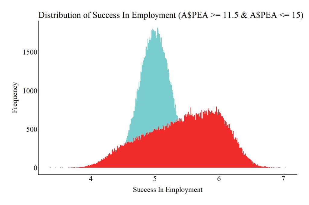
Above Average Parental Education (PEA >= 11.5 and PEA <= 15)
This time let’s sample a group of individuals with above average parental education. When the slope coefficients from the 10,000 samples of 1,000 participants with above average parental education are plotted the findings suggest that participation in the employment program causes a .40 increase in success in employment. Additionally, the sampling distribution of the difference between the treatment and control cases on success in employment (i.e., b) ranges between .30 and .55.
>N<-10000
>RSDF1 <- new.env()
>### Loop
>for(i in 1:N)
>{
>  NRS3<-sample_n(A[which(A$PEA >= 11.5 & A$PEA <= 15),] ,1000, replace = F)
>
>  LM_NRS<-lm(SIEM~EP, data = NRS3)
>  summary(LM_NRS)
>
>  NRS3DF1$Slope<-c(NRS3DF1$Slope, summary(LM_NRS)$coefficients[2])
>  NRS3DF1$SE<-c(NRS3DF1$SE, summary(LM_NRS)$coefficients[4])
>
>}

The figure below was created to illustrate the location of the above average parental education treatment and control cases. Again, pay attention to the location of the treatment distribution on the X-axis.
Below Average Parental Education (PEA >= 8 and PEA <= 11.4)
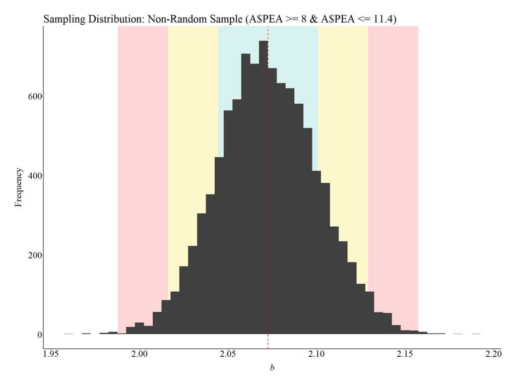
What about cases with below average parental education? Let’s draw 10,000 samples of 1,000 participants from this proportion of the distribution. When the slope coefficients from the 10,000 samples of 1,000 participants with below average parental education are plotted the findings suggest that participation in the employment program causes a 2.07 increase in success in employment. Additionally, the sampling distribution of the difference between the treatment and control cases on success in employment (i.e., b) ranges between 1.90 and 2.20.
>N<-10000
>RSDF1 <- new.env()
>### Loop
>for(i in 1:N)
>{
>  NRS4<-sample_n(A[which(A$PEA >= 8 & A$PEA <= 11.4),] ,1000, replace = F)
>
>  LM_NRS<-lm(SIEM~EP, data = NRS4)
>  summary(LM_NRS)
>
>  NRS4DF1$Slope<-c(NRS4DF1$Slope, summary(LM_NRS)$coefficients[2])
>  NRS4DF1$SE<-c(NRS4DF1$SE, summary(LM_NRS)$coefficients[4])
>
>}
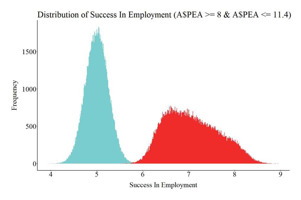
The figure below was created to illustrate the location of the below average parental education treatment and control cases.
Low Parental Education (PEA <= 8)
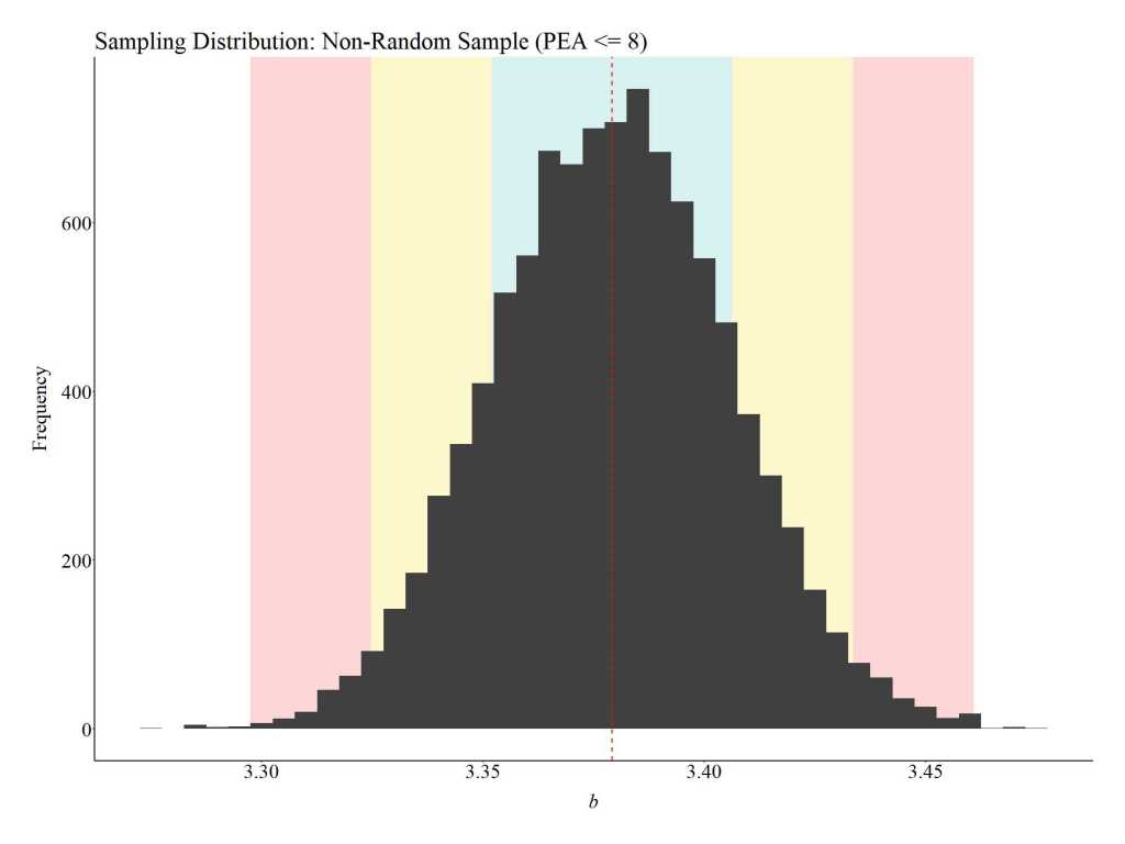
Finally, let’s take a sample of individuals with low parental education. When the slope coefficients from the 10,000 samples of 1,000 participants with low parental education are plotted the findings suggest that participation in the employment program causes a 3.37 increase in success in employment. Additionally, the sampling distribution of the difference between the treatment and control cases on success in employment (i.e., b) ranges between 3.29 and 3.50.
>N<-10000
>RSDF1 <- new.env()
>### Loop
>for(i in 1:N)
>{
>  NRS2<-sample_n(A[which(A$PEA <= 8),] ,1000, replace = F)
>
>  LM_NRS<-lm(SIEM~EP, data = NRS2)
>  summary(LM_NRS)
>
>  NRS2DF1$Slope<-c(NRS2DF1$Slope, summary(LM_NRS)$coefficients[2])
>  NRS2DF1$SE<-c(NRS2DF1$SE, summary(LM_NRS)$coefficients[4])
>
>}
The figure below was created to illustrate the location of the low parental education treatment and control cases.

Conclusion
Taken together, these findings illustrate that the effectiveness of the employment program varies by parental education. Nevertheless, when conducting a randomized controlled trial, we likely only have the time and funds to draw one sample from the population. Moreover, the cost of conducting a randomized controlled trial oftentimes encourages scholars to sacrifice the generalizability of the findings. Sacrificing the generalizability of a study is not a problem when we satisfy the assumption of known interactions. However, when an interaction between the treatment program and a third variable is unknown, drawing a convenience sample could drastically alter the perceived effectiveness of a program.
Going back to our non-random sampling distributions, if we mistakenly drew our sample from the high parental education distribution, we would perceive that the employment program is detrimental or ineffective at best. Specifically, we would conclude that individuals exposed to the employment program had lower levels of success in employment than individuals that did not participated in the employment program. In opposition, if we mistakenly drew our sample from the low parental education distribution, we would conclude that the employment program is extremely effective at increasing success in employment. While all of the non-random sampling distributions represent causal estimates (as a product of random assignment), none of the distributions captured the difference on success in employment across the entire population. Explicitly, the causal effects observed in each non-random sampling distribution would only generalize to individuals contained within that group. This highlights the potential problem with conducting experimental research on non-generalizable samples. As such, I would caution scholars to consider the effects of violating the known interaction assumption the next time they conduct a randomized controlled trial.
[i] Continuous treatment variables don’t inherently permit themselves to be examined through randomized controlled trials.
[ii] As a reminder, the focus of the series is on violating statistical assumptions. However, these assumptions also talk to methodological limitations that could exist in a randomized controlled trial.
[iii] We assume that the interaction between parental education and the employment program is unknown to us. Even though this loop is coded as a random sample, it emulates a convivence sample by only drawing cases from a proportion of the distribution on parental education.
License: Creative Commons Attribution 4.0 International (CC By 4.0)
