An outlier is a case, datapoint, or score meaningfully removed from the mass of the distribution as to be recognizably different from the remainder of cases, datapoints, or scores. Consistent with this definition, outliers are conditioned upon the observed data and can vary between samples. For example, an individual with 10 armed robberies might be an outlier in a nationally representative sample, but will likely be well within the distribution in a sample of high-risk incarcerated individuals. Consistent with the inability to explicitly define an outlier, we make no assumptions about the existence of outliers when estimating a regression model. We do, however, assume that the residual error – the difference between the predictedvalue (Yhat) and the observed value – of the dependent variable (Y) will be normally distributed (i.e., the normality assumption). The inclusion of particular outliers in a model could violate the normality assumption and introduce bias into the estimates derived from a linear regression model. The current entry reviews the effects of outliers on the estimates derived from an ordinary least squares (OLS) regression model.
Normality Assumption
Before defining the normality assumption, it is important to discuss what residuals refer to in the context of a regression model. A regression model – with different estimation procedures depending upon the model – estimates the intercept (the value of Y when X is zero) and the slope coefficient (the change in Y corresponding to a change in X) that best fits the data. Fundamentally, this is a single line used to illustrate the predicted value of the dependent variable (Yhat)at any score on the independent variable (X). This single regression line, however, is unlikely to make the appropriate prediction for the dependent variable (Y)at every value on the independent variable (X). Explicitly, Yhat (the predicted value of Y)for any one X-value is likely not going to equal the value of Y observed in the dataat the same X-value. The difference between the value of Y observed in the dataand Yhat at a specifiedvalue on the independent variable (X) is a residual. A residual is simply a method of quantifying the amount of unpredicted variation – or error – remaining after the regression model is estimated. Using this calculation, we can find the residual for each case, at each value of X, and build a distribution of residuals.
We have satisfied the normality assumption when the residuals for the dependent variable are normally distributed across the values on the independent variable (i.e., the traditional bell-curve distribution). When the residuals for the dependent variable are not normally distributed across the values on the independent variable we have violated the normality assumption. Although the normality assumption can be violated by various data peculiarities, the inclusion of outliers in our regression models represents one way we can violate the normality assumption.
The existence of outliers in a dataset – observations defined as substantively different than every other observation – can create a condition where the residuals of the dependent variable are not normally distributed across the values on the independent variable. Only certain outliers, however, can violate the normality assumption and alter the results of the regression model. In a bivariate regression model three types of outliers can exist: outlier on X only, outlier on Y only, and an outlier on X and Y. The remainder of the entry will explore how these three types of outliers can affect the slope coefficients, standard errors, and hypothesis tests conducted in an OLS regression model.
No Outliers
As we begin with every simulated exploration, let us start out by specifying a directed equation simulation that does not contain any outliers. For this example, we simply specify that we want a sample of 100 cases (N in code) with unique identifiers (ID in code). Additionally, we specify that Y is equal to .60 multiplied by X (a normally distributed variable with a mean of 10 and a SD of 1) plus .50 multiplied by a normally distributed variable with a mean of 10 and a SD of 1 (representing additional random error).[i] After specifying the data, we than create a data frame, estimate a linear OLS regression model, and plot the bivariate linear association between X and Y. The slope of the association was equal to .5934, the standard error was .0582, the standardized slope coefficient was .7174, and the association was significant at p < .001.
> N<-100
> ID<-c(1:100)
> set.seed(32)
> X<-rnorm(N,10,1)
> set.seed(15)
> Y<-.60*X+.50*rnorm(N,10,1)
>
> Data<-data.frame(ID,Y,X)
>
> M<-lm(Y~X, data = Data)
> summary(M)

Call:
lm(formula = Y ~ X, data = Data)

Residuals:
    Min      1Q  Median      3Q     Max
-1.2695 -0.3101 -0.0388  0.3855  1.1858

Coefficients:
            Estimate Std. Error t value             Pr(>|t|)
(Intercept)   5.1165     0.5806    8.81    0.000000000000045 ***
X             0.5934     0.0582   10.19 < 0.0000000000000002 ***
---
Signif. codes:  0 ‘***’ 0.001 ‘**’ 0.01 ‘*’ 0.05 ‘.’ 0.1 ‘ ’ 1

Residual standard error: 0.499 on 98 degrees of freedom
Multiple R-squared:  0.515,	Adjusted R-squared:  0.51
F-statistic:  104 on 1 and 98 DF,  p-value: <0.0000000000000002

> lm.beta(M)

Call:
lm(formula = Y ~ X, data = Data)

Standardized Coefficients::
(Intercept)           X
     0.0000      0.7174

Outliers on One Variable (X & Y) But Not the Other (N = 101) [ii]
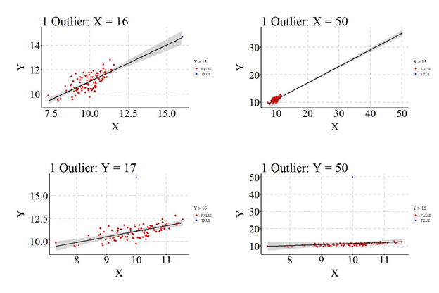
Example 1: Outliers on X but not Y (X = 16)
To simulate an outlier on X but not Y we will replicate the process for no outliers, except add a single case in the second step. Specifically, we specify an additional datapoint (ID = 101) with our desired X and Y values. For our first example, we wanted to simulate a case that is a small outlier on X but not an outlier on Y. As such, the outlying case was specified to have a value of 16 on X and a Y value with the same relationship with X as the remainder of the Y datapoints. After creating the outlier, the model is estimated and the plot was recreated (the outlier is the blue point in the scatterplot). The results of the linear OLS regression model suggested that the outlier has a slight biasing effect on the slope coefficient, downwardly biased (i.e., closer to zero) the standard error, upwardly biased (i.e., further from zero) the standardized slope coefficient (b = .5999; SE = .0474; β = .7862), and no effect on the p-value.
> ## Data
> N<-100
> ID<-c(1:100)
> set.seed(32)
> X<-rnorm(N,10,1)
> set.seed(15)
> Y<-.60*X+.50*rnorm(N,10,1)
> Data<-data.frame(ID,Y,X)
>
> ## Outlier
> ID<-101
> X<-16
> set.seed(15)
> Y<-.60*X+.50*rnorm(1,10,1)
> O<-data.frame(ID,Y,X)
>
> D_O<-rbind(Data,O)
>
> M<-lm(Y~X, data = D_O)
> summary(M)

Call:
lm(formula = Y ~ X, data = D_O)

Residuals:
    Min      1Q  Median      3Q     Max
-1.2707 -0.3116 -0.0405  0.3757  1.1906

Coefficients:
            Estimate Std. Error t value            Pr(>|t|)
(Intercept)   5.0532     0.4762    10.6 <0.0000000000000002 ***
X             0.5999     0.0474    12.7 <0.0000000000000002 ***
---
Signif. codes:  0 ‘***’ 0.001 ‘**’ 0.01 ‘*’ 0.05 ‘.’ 0.1 ‘ ’ 1

Residual standard error: 0.497 on 99 degrees of freedom
Multiple R-squared:  0.618,	Adjusted R-squared:  0.614
F-statistic:  160 on 1 and 99 DF,  p-value: <0.0000000000000002

> lm.beta(M)

Call:
lm(formula = Y ~ X, data = D_O)

Standardized Coefficients::
(Intercept)           X
     0.0000      0.7862
Example 2: Outliers on X but not Y (X = 50)
For the second example, our outlying case was specified to have a value of 50 on X and a Y value with the same relationship with X as the remainder of the Y datapoints (N = 101). Presented below are the results corresponding to the estimated linear OLS regression model. The results illustrated, similar to the previous example, that the outlier on only X had a slight biasing effect on the slope coefficient, downwardly biased the standard error, upwardly biased the standardized slope coefficient (b = .6016; SE = .0122; β = .9803), and no effect on the p-value.
> ## Data
> N<-100
> ID<-c(1:100)
> set.seed(32)
> X<-rnorm(N,10,1)
> set.seed(15)
> Y<-.60*X+.50*rnorm(N,10,1)
> Data<-data.frame(ID,Y,X)
>
> ## Outlier
> ID<-101
> X<-50
> set.seed(15)
> Y<-.60*X+.50*rnorm(1,10,1)
> O<-data.frame(ID,Y,X)
> D_O<-rbind(Data,O)
>
> M<-lm(Y~X, data = D_O)
> summary(M)

Call:
lm(formula = Y ~ X, data = D_O)

Residuals:
    Min      1Q  Median      3Q     Max
-1.2701 -0.3125 -0.0404  0.3754  1.1927

Coefficients:
            Estimate Std. Error t value            Pr(>|t|)
(Intercept)   5.0356     0.1353    37.2 <0.0000000000000002 ***
X             0.6016     0.0122    49.4 <0.0000000000000002 ***
---
Signif. codes:  0 ‘***’ 0.001 ‘**’ 0.01 ‘*’ 0.05 ‘.’ 0.1 ‘ ’ 1

Residual standard error: 0.497 on 99 degrees of freedom
Multiple R-squared:  0.961,	Adjusted R-squared:  0.961
F-statistic: 2.44e+03 on 1 and 99 DF,  p-value: <0.0000000000000002

> lm.beta(M)

Call:
lm(formula = Y ~ X, data = D_O)

Standardized Coefficients::
(Intercept)           X
     0.0000      0.9803
Example 3: Outliers on Y but not X (Y = 17; X = 10 [mean of X])
After exploring how outliers on X but not Y influenced our estimated coefficients, we must explore how outliers on Y but not X influence the estimated coefficients. For the third example, we replicated the above specification except the X and Y values for the outlier were specified to be 10 (the mean of X) and 17, respectively. The results of the OLS regression model, again, illustrated that the outlier on Y but not X only slightly biased the slope coefficient, upwardly biased the standard error, downwardly biased the standardized slope coefficient (b = .5986; SE = .0904; β = .5542), and no effect on the p-value.
> ## Data
> N<-100
> ID<-c(1:100)
> set.seed(32)
> X<-rnorm(N,10,1)
> set.seed(15)
> Y<-.60*X+.50*rnorm(N,10,1)
> Data<-data.frame(ID,Y,X)
>
> ## Outlier
> ID<-101
> X<-10
> set.seed(15)
> Y<-17
> O<-data.frame(ID,Y,X)
> D_O<-rbind(Data,O)
>
> M<-lm(Y~X, data = D_O)
> summary(M)

Call:
lm(formula = Y ~ X, data = D_O)

Residuals:
   Min     1Q Median     3Q    Max
-1.329 -0.369 -0.098  0.340  5.890

Coefficients:
            Estimate Std. Error t value     Pr(>|t|)
(Intercept)   5.1243     0.9011    5.69 0.0000001313 ***
X             0.5986     0.0904    6.62 0.0000000018 ***
---
Signif. codes:  0 ‘***’ 0.001 ‘**’ 0.01 ‘*’ 0.05 ‘.’ 0.1 ‘ ’ 1

Residual standard error: 0.775 on 99 degrees of freedom
Multiple R-squared:  0.307,	Adjusted R-squared:   0.3
F-statistic: 43.9 on 1 and 99 DF,  p-value: 0.00000000183

> lm.beta(M)

Call:
lm(formula = Y ~ X, data = D_O)

Standardized Coefficients::
(Intercept)           X
     0.0000      0.5542
Example 4: Outliers on Y but not X (Y = 50; X = 10 [mean of X])
This process was replicated again, except the outlier was specified to have a value of 50 for Y (X remained 10). After simulating the data, our linear OLS regression model was reestimated. The results, as you can now expect, illustrated that the inclusion of the outlier in our analytical sample slightly biased the slope coefficient, upwardly biased the standard error, downwardly biased the standardized slope coefficient (b = .6271; SE = .4577; β = .1364) and downwardly biased the p-value (p > .05).
> ## Data
> N<-100
> ID<-c(1:100)
> set.seed(32)
> X<-rnorm(N,10,1)
> set.seed(15)
> Y<-.60*X+.50*rnorm(N,10,1)
> Data<-data.frame(ID,Y,X)
>
> ## Outlier
> ID<-101
> X<-10
> set.seed(15)
> Y<-50
> O<-data.frame(ID,Y,X)
> D_O<-rbind(Data,O)
>
> M<-lm(Y~X, data = D_O)
> print(summary(M), digits = 4)

Call:
lm(formula = Y ~ X, data = D_O)

Residuals:
   Min     1Q Median     3Q    Max
-1.657 -0.717 -0.433 -0.008 38.562

Coefficients:
            Estimate Std. Error t value Pr(>|t|)
(Intercept)   5.1674     4.5642   1.132    0.260
X             0.6271     0.4577   1.370    0.174

Residual standard error: 3.927 on 99 degrees of freedom
Multiple R-squared:  0.01861,	Adjusted R-squared:  0.0087
F-statistic: 1.878 on 1 and 99 DF,  p-value: 0.1737

> lm.beta(M)

Call:
lm(formula = Y ~ X, data = D_O)

Standardized Coefficients::
(Intercept)           X
     0.0000      0.1364
Outlier on X and Y at Ybar (N = 101)
You might have been asking yourself – as we went through the above examples – why did we not just set the Y value to the mean when exploring outliers on X but not Y (i.e., examples 1 and 2)? While that would be logical, specifying an X outlier at the mean of Y (Ybar) will commonly downwardly bias the slope coefficient of a regression line. This downward bias occurs because while Y is not an outlier, we still violate the normality assumption (i.e., the residual distribution of Y values is not normally distributed). Let’s explore this using two examples. While these examples employ a positive association, I encourage readers to use the available R-code to observe how X outlier at the mean of Y can downwardly bias negative associations (make the association closer to zero than reality).
Example 5: X = 16; Y = Ybar
Consistent with the previous examples, we replicated the no outlier code except added a single outlier (ID: 101) to the data frame that was specified to have a value of 16 on X and 11.01 (Ybar) on Y. After creating the sample, we replicated the linear OLS regression model. Distinct from the previous examples, however, the slope coefficient is downwardly biased (b = .3970) compared to the true slope coefficient (.5934). The downward bias in the slope coefficient becomes more substantial, however, when the X value is increased.
> ## Data
> N<-100
> ID<-c(1:100)
> set.seed(32)
> X<-rnorm(N,10,1)
> set.seed(15)
> Y<-.60*X+.50*rnorm(N,10,1)
> Data<-data.frame(ID,Y,X)
>
> ## Outlier
> ID<-101
> X<-16
> set.seed(15)
> Y<-mean(Y)
> O<-data.frame(ID,Y,X)
> D_O<-rbind(Data,O)
>
> M<-lm(Y~X, data = D_O)
> summary(M)

Call:
lm(formula = Y ~ X, data = D_O)

Residuals:
    Min      1Q  Median      3Q     Max
-2.3838 -0.3676 -0.0247  0.4197  1.3037

Coefficients:
            Estimate Std. Error t value             Pr(>|t|)
(Intercept)   7.0440     0.5534   12.73 < 0.0000000000000002 ***
X             0.3970     0.0551    7.21        0.00000000011 ***
---
Signif. codes:  0 ‘***’ 0.001 ‘**’ 0.01 ‘*’ 0.05 ‘.’ 0.1 ‘ ’ 1

Residual standard error: 0.578 on 99 degrees of freedom
Multiple R-squared:  0.344,	Adjusted R-squared:  0.338
F-statistic:   52 on 1 and 99 DF,  p-value: 0.000000000113

> lm.beta(M)

Call:
lm(formula = Y ~ X, data = D_O)

Standardized Coefficients::
(Intercept)           X
     0.0000      0.5868
Example 6: X = 50; Y = Ybar
When the outlying case is specified to have a value of 50 on X and 11.01 (Ybar) on Y, the slope coefficient estimated using the simulated data is .0263 and is no longer statistically significant. Moreover, the standardized slope coefficient from the model was equal to .1509, which is a meaningful departure from the true standardized slope coefficient of .7174.
> ## Data
> N<-100
> ID<-c(1:100)
> set.seed(32)
> X<-rnorm(N,10,1)
> set.seed(15)
> Y<-.60*X+.50*rnorm(N,10,1)
> Data<-data.frame(ID,Y,X)
>
> ## Outlier
> ID<-101
> X<-50
> set.seed(15)
> Y<-mean(Y)
> O<-data.frame(ID,Y,X)
> D_O<-rbind(Data,O)
>
> M<-lm(Y~X, data = D_O)
> summary(M)

Call:
lm(formula = Y ~ X, data = D_O)

Residuals:
   Min     1Q Median     3Q    Max
-1.520 -0.528  0.080  0.516  1.800

Coefficients:
            Estimate Std. Error t value            Pr(>|t|)
(Intercept)  10.7411     0.1919   55.96 <0.0000000000000002 ***
X             0.0263     0.0173    1.52                0.13
---
Signif. codes:  0 ‘***’ 0.001 ‘**’ 0.01 ‘*’ 0.05 ‘.’ 0.1 ‘ ’ 1

Residual standard error: 0.705 on 99 degrees of freedom
Multiple R-squared:  0.0228,	Adjusted R-squared:  0.0129
F-statistic: 2.31 on 1 and 99 DF,  p-value: 0.132

> lm.beta(M)

Call:
lm(formula = Y ~ X, data = D_O)

Standardized Coefficients::
(Intercept)           X
     0.0000      0.1509

Consistent with the two examples above, the slope coefficient will commonly be downwardly biased – closer to zero – if a case is an outlier on X at Ybar. As such, outliers on X at Ybar can only serve to downwardly bias the unstandardized and standardized slope coefficients.
Outlier on X and Y (N = 101)
Finally, let’s explore the effects of an outlier on both X and Y on the estimates derived from a linear OLS regression model. In the first example we specified that the outlier would have a value of 16 on X and 20 on Y, in the second example we specified that the outlier would have a value of 50 on X and 100 on Y, in the third example we specified that the outlier would have a value of 16 on X and -25 on Y. When the outlier was specified to exist at 16on X and 25 on Y the slope of the association estimated using an OLS regression model was upwardly biased (b = 1.16), as well as the standardized slope estimate (β = .7791). When the outlier possessed a value of 50 on X and 100 on Y, the degree of upward bias was substantially increased. Specifically, the estimated slope coefficient was 2.149 and the standardized slope coefficient was .9866. Finally, when the outlier was specified to exist at 16 on X and -25 on Y the slope of the association estimated using an OLS regression model was upwardly biased (further from zero) but the sign was flipped (b = -1.586), as well as the standardized slope estimate (β = -.4503). Overall, a common outlier on X and Y will frequently upwardly bias the slope coefficient.
Example 7: X = 16; Y = 25
> ## Data
> N<-100
> ID<-c(1:100)
> set.seed(32)
> X<-rnorm(N,10,1)
> set.seed(15)
> Y<-.60*X+.50*rnorm(N,10,1)
> Data<-data.frame(ID,Y,X)
>
> ## Outlier
> ID<-101
> X<-16
> set.seed(15)
> Y<-25
> O<-data.frame(ID,Y,X)
> D_O<-rbind(Data,O)
>
> M<-lm(Y~X, data = D_O)
> summary(M)

Call:
lm(formula = Y ~ X, data = D_O)

Residuals:
   Min     1Q Median     3Q    Max
-1.369 -0.600 -0.092  0.463  6.882

Coefficients:
            Estimate Std. Error t value            Pr(>|t|)
(Intercept)  -0.4478     0.9432   -0.47                0.64
X             1.1604     0.0939   12.36 <0.0000000000000002 ***
---
Signif. codes:  0 ‘***’ 0.001 ‘**’ 0.01 ‘*’ 0.05 ‘.’ 0.1 ‘ ’ 1

Residual standard error: 0.984 on 99 degrees of freedom
Multiple R-squared:  0.607,	Adjusted R-squared:  0.603
F-statistic:  153 on 1 and 99 DF,  p-value: <0.0000000000000002

> lm.beta(M)

Call:
lm(formula = Y ~ X, data = D_O)

Standardized Coefficients::
(Intercept)           X
     0.0000      0.7791
Example 8: X = 50; Y = 100
> ## Data
> N<-100
> ID<-c(1:100)
> set.seed(32)
> X<-rnorm(N,10,1)
> set.seed(15)
> Y<-.60*X+.50*rnorm(N,10,1)
> Data<-data.frame(ID,Y,X)
>
> ## Outlier
> ID<-101
> X<-50
> set.seed(15)
> Y<-100
> O<-data.frame(ID,Y,X)
> D_O<-rbind(Data,O)
>
> M<-lm(Y~X, data = D_O)
> summary(M)

Call:
lm(formula = Y ~ X, data = D_O)

Residuals:
   Min     1Q Median     3Q    Max
-2.285 -1.164 -0.132  0.919  4.500

Coefficients:
            Estimate Std. Error t value            Pr(>|t|)
(Intercept) -10.3113     0.3973     -26 <0.0000000000000002 ***
X             2.1491     0.0358      60 <0.0000000000000002 ***
---
Signif. codes:  0 ‘***’ 0.001 ‘**’ 0.01 ‘*’ 0.05 ‘.’ 0.1 ‘ ’ 1

Residual standard error: 1.46 on 99 degrees of freedom
Multiple R-squared:  0.973,	Adjusted R-squared:  0.973
F-statistic: 3.61e+03 on 1 and 99 DF,  p-value: <0.0000000000000002

> lm.beta(M)

Call:
lm(formula = Y ~ X, data = D_O)

Standardized Coefficients::
(Intercept)           X
     0.0000      0.9866
Example 9: X = 16; Y = -25
> ## Data
> N<-100
> ID<-c(1:100)
> set.seed(32)
> X<-rnorm(N,10,1)
> set.seed(15)
> Y<-.60*X+.50*rnorm(N,10,1)
> Data<-data.frame(ID,Y,X)
>
>
>
> ## Outlier
> ID<-101
> X<-16
> set.seed(15)
> Y<--25
> O<-data.frame(ID,Y,X)
>
> D_O<-rbind(Data,O)
>
> M<-lm(Y~X, data = D_O)
> summary(M)

Call:
lm(formula = Y ~ X, data = D_O)

Residuals:
    Min      1Q  Median      3Q     Max
-26.239  -1.019   0.407   1.644   4.243

Coefficients:
            Estimate Std. Error t value         Pr(>|t|)
(Intercept)   26.333      3.141    8.38 0.00000000000036 ***
X             -1.568      0.313   -5.02 0.00000229958141 ***
---
Signif. codes:  0 ‘***’ 0.001 ‘**’ 0.01 ‘*’ 0.05 ‘.’ 0.1 ‘ ’ 1

Residual standard error: 3.28 on 99 degrees of freedom
Multiple R-squared:  0.203,	Adjusted R-squared:  0.195
F-statistic: 25.2 on 1 and 99 DF,  p-value: 0.0000023

> lm.beta(M)

Call:
lm(formula = Y ~ X, data = D_O)

Standardized Coefficients::
(Intercept)           X
     0.0000     -0.4503

Conclusions
This entry explored the effects of outliers at different locations on the slope coefficients, standard errors, standardized slope coefficients, and p-values from linear OLS regression models. As demonstrated: (1) outliers on X but not Y will only result in slight biases to the estimates from a regression model, (2) outliers on Y but not X will only result in slight biases to the estimates from a regression model , (3) outliers on X but within the distribution of Y will commonly downwardly bias the unstandardized and standardized slope coefficients, (4) and outliers on both X and Y will commonly upwardly bias the unstandardized and standardized slope coefficients.[iii] While discussing the effects of potential outliers is important when reviewing the results of a regression model, only an outlier on both X and Y can result in meaningful upward bias in the unstandardized and standardized slope coefficients and, in turn, increase the likelihood of rejecting the null hypothesis when the null hypothesis should have been retained. Moreover, the effects of an outlier on both X and Y depends upon the sample size (Illustrated in the available R-Code). As such, sensitivity analyses should be estimated to explore if an outlier on both X and Y exists in the sample and the effects of the outlier on the estimated coefficients. If the effects are statistically significant when the outlier is included and not statistically significant when the outlier is excluded, justification should be provided for the differences between the models.
I, however, believe it is important to remind readers about the caution that has to exist when handling outliers in a dataset. Primarily, a datapoint is recognizably different from the remainder of the distribution for three reasons: (1) measurement error, (2) random error, and (3) these datapoints exist in the broader population. All three present difficulties for defining and handling outliers. The existence of known measurement error represents the situation where outliers are the easiest to handle. Specifically, if scores are unreasonable, unlikely, or not realistic we can justifiably remove those cases from the data due to the inability to properly score particular cases. Nevertheless, if there is no apparent measurement error, the regression model estimated without an outlier included could be more biased – further from the population estimates – than the regression model estimated with the outlier included. Moreover, the removal of multiple datapoints perceived as outliers could meaningfully alter the results of the model. Considering this, extreme caution should be taken when evaluating if it is or is not appropriate to remove perceived outliers from a dataset prior to estimating a regression model. Only in undoubtedly justifiable circumstances should you non-randomly remove perceived outliers from a dataset.[iv]
[i] The inclusion of random error ensures that values on X do not perfectly predict values on Y.
[ii] All of the examples below are replicated in the R-code with 1,001 and 10,001 cases.
[iii] In addition to the examples reviewed above, the available R-code also replicates the examples using samples comprised of 1,001 and 10,001 cases.
[iv] The effects of non-randomly removing cases from a dataset will be reviewed when discussing additional assumptions of regression models.
License: Creative Commons Attribution 4.0 International (CC By 4.0)
