Regression based techniques are one of the most frequently used statistical approaches for hypothesis testing. The primary benefit of regression techniques is the ability to adjust estimates for the variation across multiple independent variables – otherwise known as the statistical control approach. This is extremely valuable when we are interested in the relationship between an independent variable and a dependent variable, but are unable to conduct a randomized controlled trial (i.e., true experiment). However, when introducing numerous statistical controls into a regression model we make assumptions about the structure of the variation across the independent variables. One assumption is that the independent variables are only highly correlated with the dependent variable. To state differently, we assume that multicollinearity – high levels of intercorrelation – does not exist across the independent variables. The current entry will illustrate how violating this assumption, and the degree of the violation, affect our estimates produced by OLS regression models.
Defining Statistical Controls and Multicollinearity
Before defining multicollinearity, it is important to review how the statistical control method works. In a traditional bivariate regression model, we are interested in estimating if variation in X predicts variation in Y and the strength of that prediction. Ordinary least squares regression – the most frequently used linear regression model – estimates an association by calculating a linear regression line where the predicted x,y point is as close as possible to every observed x,y point in the scatterplot. When a statistical control is introduced into a model, the linear regression line is altered by removing variation in Y predicted by variation in Z or variation in X predicted by Z. This means that observed x,y points that correspond with y,z points or x,z pointsare no longer included in the calculation of the linear regression line. To state differently, all of the cases where values of Y correlate with values of Z or values of X correlate with values of Z are removed from the calculation of the linear regression line. By removing these points – or cases – we can adjust our linear regression line for the influence of Z and increase our ability to estimate the true association between X and Y. Through this simplistic description of statistical controls, we can now define multicollinearity in the context of statistical controls. Multicollinearity is defined as the observation of a noticeable degree of correspondence between the variation in two or more independent variables. In this sense, multicollinearity is a special condition of a correlation, where Z1 through Zk (or X1 through Xk) are highly intercorrelated.
When using the statistical control method, we assume that variation in a control variable predicts variation in the dependent variable (Y), which by adjusting for increases our ability to estimate the true association between X and Y. When including multiple control variables, we assume that the variation in Z1through Zk. predicts variation in Y, but is not highly correlated with variation in X or variation in Z1 through Zk. This assumption, however, can be violated when Z1 through Zk are highly correlated with X and highly correlated with each other. As demonstrated in this entry, violating this assumption means that we can not estimate the true association between X and Y when Z1 through Zk are included as statistical controls in the regression model.
Simulation 1: No Intercorrelation
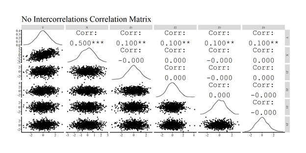
Let’s start by discussing a simulation where variation in the control variables only predict variation in Y. Due to the need to simulate intercorrelated data, we will rely on the matrix-based simulation technique. Matrix-based simulations will create intercorrelated data that is consistent with a correlation matrix provided by the user. Specifically, we will simply provide R with a correlation matrix and R will simulate data that produces the specified correlation matrix. For the current simulation, our correlation matrix will be specified where the first row and column correspond to the dependent variable (Y), the second row and column correspond to the independent variable of interest (X), and the remaining four rows and columns will correspond to the control variables (Z1–Z4). Consistent with a correlation matrix, each cell in the diagonal of the matrix is specified as 1 and all corresponding cells above and below the diagonal are identical.
To create an association between X and Y, the cells corresponding to row 1 column 2 and row 2 column 1 will be specified to have a correlation of .50. The remaining cells in row 1 and column 1 are specified to have a correlation of .10, which means that Z1–Z4 will each a correlation of .10 with Y. The remaining cells receive a 0 to ensure that none of the independent variables – X and Z1–Z4 – are correlated with each other. After specifying the matrix, we simulate the data using the mvrnorm command (from the MASS package), where n is the number of cases (n = 1000), mu is the mean of the variables (mu = 0 for each variable), Sigma is the specified correlation matrix (Sigma = CM), and empirical informs R to not deviate from the specified correlation matrix (empirical = TRUE). After simulating the data, we use the tidyverse package to rename the columns to our desired specifications.
CM<-matrix(c(1,.50,.10,.10,.10,.10,
             .50,1,.0,.0,.0,.0,
             .10,.0,1,0,0,0,
             .10,.0,0,1,0,0,
             .10,.0,0,0,1,0,
             .10,.0,0,0,0,1), nrow = 6)

set.seed(56)
DF<-data.frame(mvrnorm(n = 1000, mu = rep(0, 6), Sigma = CM, empirical = TRUE))

DF<-DF %>%
  rename(
    Y = X1,
    X = X2,
    Z1 = X3,
    Z2 = X4,
    Z3 = X5,
    Z4 = X6
  )
For illustrative purposes, we then use GGally in combination with ggplot2 to create a visual correlation matrix. As observed, the simulated data has a correlation matrix identical to our specification of the data.
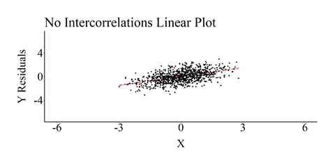
After producing the correlation matrix, we will estimate an ordinary least squares (OLS) regression model where Y is regressed on X and Z1–Z4. The results of the model are consistent with our specification, where the estimated slope of the association between X and Y is .50 and the estimated slope of the associations between Z1–Z4 and Y are .10. The resulting slope coefficients are consistent with the specification of the simulation because the mean of every construct is 0 and the standard deviation is 1. We then created a scatterplot of the association, including the linear regression line, between X and Y (Residuals)after adjusting for Z1 through Z4.[i]
> M<-lm(Y~X+Z1+Z2+Z3+Z4, data = DF)
>
> summary(M)

Call:
lm(formula = Y ~ X + Z1 + Z2 + Z3 + Z4, data = DF)

Residuals:
   Min     1Q Median     3Q    Max
-2.743 -0.569  0.010  0.522  2.264

Coefficients:
                          Estimate             Std. Error t value             Pr(>|t|)
(Intercept) -0.0000000000000000214  0.0267127577867098606    0.00              1.00000
X            0.5000000000000003331  0.0267261241912424390   18.71 < 0.0000000000000002 ***
Z1           0.0999999999999996170  0.0267261241912424286    3.74              0.00019 ***
Z2           0.1000000000000000611  0.0267261241912424320    3.74              0.00019 ***
Z3           0.1000000000000002137  0.0267261241912424494    3.74              0.00019 ***
Z4           0.0999999999999996586  0.0267261241912424112    3.74              0.00019 ***
---
Signif. codes:  0 ‘***’ 0.001 ‘**’ 0.01 ‘*’ 0.05 ‘.’ 0.1 ‘ ’ 1

Residual standard error: 0.845 on 994 degrees of freedom
Multiple R-squared:  0.29,	Adjusted R-squared:  0.286
F-statistic: 81.2 on 5 and 994 DF,  p-value: <0.0000000000000002

> lm.beta(M)

Call:
lm(formula = Y ~ X + Z1 + Z2 + Z3 + Z4, data = DF)

Standardized Coefficients::
(Intercept)           X          Z1          Z2          Z3          Z4
        0.0         0.5         0.1         0.1         0.1         0.1

> ols_coll_diag(M)
Tolerance and Variance Inflation Factor
---------------------------------------
  Variables Tolerance VIF
1         X         1   1
2        Z1         1   1
3        Z2         1   1
4        Z3         1   1
5        Z4         1   1


Eigenvalue and Condition Index
------------------------------
  Eigenvalue Condition Index intercept        X       Z1        Z2       Z3     Z4
1          1               1         0 0.002163 0.942058 0.0009771 0.038598 0.0162
2          1               1         0 0.141103 0.040010 0.0202728 0.455664 0.3429
3          1               1         0 0.029184 0.000000 0.5818457 0.197989 0.1910
4          1               1         1 0.000000 0.000000 0.0000000 0.000000 0.0000
5          1               1         0 0.575826 0.009721 0.1730437 0.003303 0.2381
6          1               1         0 0.251724 0.008211 0.2238607 0.304446 0.2118
As demonstrated in the above simulation, the association between X and Y is not biased when Z1–Z4 are included in the regression model. This is because the independent variables – X and Z1–Z4 – satisfy the assumption that variation in the control variables only predict variation in Y.
Simulation 2: Small Intercorrelation
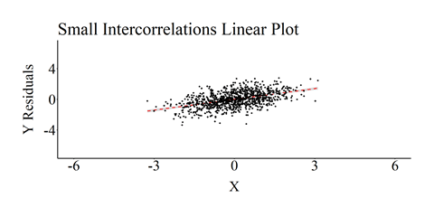
For our second simulation, we will replicate the first simulation except slightly increase the correlation among the independent variables (X and Z1–Z4). Specifically, in the first simulation we specified that X and Z1–Z4 were uncorrelated, while in the second simulation we indicate that X and Z1–Z4 are intercorrelated at .10 (i.e., every cell containing a zero in the previous simulation was specified to be .10 in the current simulation). Importantly, the relationship between X and Y was specified to be .50. The visual correlation matrix was then recreated. The correlation matrix of the simulated data perfectly matched our specifications.
CM<-matrix(c(1,.50,.10,.10,.10,.10,
             .50,1,.10,.10,.10,.10,
             .10,.10,1,.10,.10,.10,
             .10,.10,.10,1,.10,.10,
             .10,.10,.10,.10,1,.10,
             .10,.10,.10,.10,.10,1), nrow = 6)

set.seed(56)
DF<-data.frame(mvrnorm(n = 1000, mu = rep(0, 6), Sigma = CM, empirical = TRUE))

DF<-DF %>%
  rename(
    Y = X1,
    X = X2,
    Z1 = X3,
    Z2 = X4,
    Z3 = X5,
    Z4 = X6
  )

The OLS regression model was then reestimated and we recreated a scatterplot of the association, including the linear regression line, between X and Y (Residuals)after adjusting for Z1 through Z4. Although not a noticeable deviation from the specification, the estimated association between X and Y was .484 (not .50 like the specification).
> M<-lm(Y~X+Z1+Z2+Z3+Z4, data = DF)
>
> summary(M)

Call:
lm(formula = Y ~ X + Z1 + Z2 + Z3 + Z4, data = DF)

Residuals:
   Min     1Q Median     3Q    Max
-3.254 -0.593 -0.011  0.570  2.594

Coefficients:
                          Estimate             Std. Error t value            Pr(>|t|)
(Intercept) -0.0000000000000000471  0.0273092695948878271    0.00                1.00
X            0.4841269841269854601  0.0277532433843363582   17.44 <0.0000000000000002 ***
Z1           0.0396825396825397497  0.0277532433843363478    1.43                0.15
Z2           0.0396825396825404228  0.0277532433843363860    1.43                0.15
Z3           0.0396825396825400828  0.0277532433843363513    1.43                0.15
Z4           0.0396825396825398885  0.0277532433843363929    1.43                0.15
---
Signif. codes:  0 ‘***’ 0.001 ‘**’ 0.01 ‘*’ 0.05 ‘.’ 0.1 ‘ ’ 1

Residual standard error: 0.864 on 994 degrees of freedom
Multiple R-squared:  0.258,	Adjusted R-squared:  0.254
F-statistic: 69.1 on 5 and 994 DF,  p-value: <0.0000000000000002

> lm.beta(M)

Call:
lm(formula = Y ~ X + Z1 + Z2 + Z3 + Z4, data = DF)

Standardized Coefficients::
(Intercept)           X          Z1          Z2          Z3          Z4
    0.00000     0.48413     0.03968     0.03968     0.03968     0.03968

> ols_coll_diag(M)
Tolerance and Variance Inflation Factor
---------------------------------------
  Variables Tolerance   VIF
1         X    0.9692 1.032
2        Z1    0.9692 1.032
3        Z2    0.9692 1.032
4        Z3    0.9692 1.032
5        Z4    0.9692 1.032


Eigenvalue and Condition Index
------------------------------
  Eigenvalue Condition Index intercept        X      Z1      Z2       Z3         Z4
1        1.4           1.000         0 0.138462 0.13846 0.13846 0.138462 0.13846154
2        1.0           1.183         1 0.000000 0.00000 0.00000 0.000000 0.00000000
3        0.9           1.247         0 0.734130 0.25952 0.03559 0.002818 0.04486554
4        0.9           1.247         0 0.114162 0.45025 0.18589 0.326582 0.00003915
5        0.9           1.247         0 0.011382 0.03619 0.52447 0.500425 0.00445671
6        0.9           1.247         0 0.001864 0.11558 0.11558 0.031714 0.81217706
The effects, however, become more noticeable as the intercorrelation between the independent variables increase.
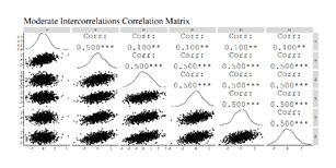
Simulations 3-5: Moderately Small, Moderate, and High Intercorrelation
For the remaining simulations – moderately small, moderate, and high –, we increased the correlations amongst the independent variables to .25, .50, and .75 (respectively). The code for the remaining simulations is identical to the previous simulations except for altering the correlation matrix specification amongst the independent variables.
Moderately Small Intercorrelation Simulation Code
CM<-matrix(c(1,.50,.10,.10,.10,.10,
             .50,1,.25,.25,.25,.25,
             .10,.25,1,.25,.25,.25,
             .10,.25,.25,1,.25,.25,
             .10,.25,.25,.25,1,.25,
             .10,.25,.25,.25,.25,1), nrow = 6)

set.seed(56)
DF<-data.frame(mvrnorm(n = 1000, mu = rep(0, 6), Sigma = CM, empirical = TRUE))


DF<-DF %>%
  rename(
    Y = X1,
    X = X2,
    Z1 = X3,
    Z2 = X4,
    Z3 = X5,
    Z4 = X6
  )
Moderate Intercorrelation Simulation Code
CM<-matrix(c(1,.50,.10,.10,.10,.10,
             .50,1,.50,.50,.50,.50,
             .10,.50,1,.50,.50,.50,
             .10,.50,.50,1,.50,.50,
             .10,.50,.50,.50,1,.50,
             .10,.50,.50,.50,.50,1), nrow = 6)

set.seed(56)
DF<-data.frame(mvrnorm(n = 1000, mu = rep(0, 6), Sigma = CM, empirical = TRUE))

DF<-DF %>%
  rename(
    Y = X1,
    X = X2,
    Z1 = X3,
    Z2 = X4,
    Z3 = X5,
    Z4 = X6
  )
High Intercorrelation Simulation Code
CM<-matrix(c(1,.50,.10,.10,.10,.10,
             .50,1,.75,.75,.75,.75,
             .10,.75,1,.75,.75,.75,
             .10,.75,.75,1,.75,.75,
             .10,.75,.75,.75,1,.75,
             .10,.75,.75,.75,.75,1), nrow = 6)

set.seed(56)
DF<-data.frame(mvrnorm(n = 1000, mu = rep(0, 6), Sigma = CM, empirical = TRUE))

DF<-DF %>%
  rename(
    Y = X1,
    X = X2,
    Z1 = X3,
    Z2 = X4,
    Z3 = X5,
    Z4 = X6
  )
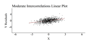
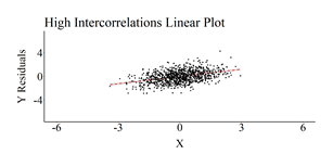
The correlation matrices were then produced, the OLS regression models were estimated, and scatterplots of the association between X and Y (Residuals)after adjusting for Z1 through Z4 were created. The results of the regression model estimated on the simulated data with moderately small intercorrelation demonstrated only a slight upward bias (Estimated b = .52; True b = .50). Nevertheless, the regression model estimated using the simulated data with moderate intercorrelation demonstrated a .20 upward departure from the true slope coefficient (Estimated b = .70; True b = .50) and the regression model estimated using the simulated data with high intercorrelation demonstrated a .82 upward departure from the true slope coefficient (Estimated b = 1.32; True b = .50).
Moderately Small Intercorrelation Results
> M<-lm(Y~X+Z1+Z2+Z3+Z4, data = DF)
>
> summary(M)

Call:
lm(formula = Y ~ X + Z1 + Z2 + Z3 + Z4, data = DF)

Residuals:
   Min     1Q Median     3Q    Max
-3.612 -0.588 -0.009  0.562  2.712

Coefficients:
                          Estimate             Std. Error t value            Pr(>|t|)
(Intercept) -0.0000000000000000249  0.0274243976326386460    0.00                1.00
X            0.5166666666666698271  0.0296365569627647200   17.43 <0.0000000000000002 ***
Z1          -0.0166666666666668468  0.0296365569627647027   -0.56                0.57
Z2          -0.0166666666666665277  0.0296365569627646611   -0.56                0.57
Z3          -0.0166666666666659656  0.0296365569627647166   -0.56                0.57
Z4          -0.0166666666666670966  0.0296365569627646680   -0.56                0.57
---
Signif. codes:  0 ‘***’ 0.001 ‘**’ 0.01 ‘*’ 0.05 ‘.’ 0.1 ‘ ’ 1

Residual standard error: 0.867 on 994 degrees of freedom
Multiple R-squared:  0.252,	Adjusted R-squared:  0.248
F-statistic: 66.9 on 5 and 994 DF,  p-value: <0.0000000000000002

> lm.beta(M)

Call:
lm(formula = Y ~ X + Z1 + Z2 + Z3 + Z4, data = DF)

Standardized Coefficients::
(Intercept)           X          Z1          Z2          Z3          Z4
    0.00000     0.51667    -0.01667    -0.01667    -0.01667    -0.01667

> ols_coll_diag(M)
Tolerance and Variance Inflation Factor
---------------------------------------
  Variables Tolerance   VIF
1         X    0.8571 1.167
2        Z1    0.8571 1.167
3        Z2    0.8571 1.167
4        Z3    0.8571 1.167
5        Z4    0.8571 1.167


Eigenvalue and Condition Index
------------------------------
  Eigenvalue Condition Index intercept         X      Z1      Z2      Z3        Z4
1       2.00           1.000         0 0.0857143 0.08571 0.08571 0.08571 0.0857143
2       1.00           1.414         1 0.0000000 0.00000 0.00000 0.00000 0.0000000
3       0.75           1.633         0 0.0003314 0.10090 0.45241 0.10440 0.4848087
4       0.75           1.633         0 0.6203864 0.36620 0.13077 0.02507 0.0004327
5       0.75           1.633         0 0.2201670 0.41516 0.04601 0.07849 0.3830299
6       0.75           1.633         0 0.0734010 0.03202 0.28509 0.70633 0.0460144


Moderate Intercorrelation Results
> M<-lm(Y~X+Z1+Z2+Z3+Z4, data = DF)
>
> summary(M)

Call:
lm(formula = Y ~ X + Z1 + Z2 + Z3 + Z4, data = DF)

Residuals:
    Min      1Q  Median      3Q     Max
-2.9677 -0.5623 -0.0094  0.5669  3.0278

Coefficients:
                         Estimate            Std. Error t value            Pr(>|t|)
(Intercept) -0.000000000000000153  0.026333834224239020    0.00              1.0000
X            0.699999999999995182  0.034013844973766146   20.58 <0.0000000000000002 ***
Z1          -0.099999999999999326  0.034013844973766215   -2.94              0.0034 **
Z2          -0.099999999999998465  0.034013844973766263   -2.94              0.0034 **
Z3          -0.099999999999998618  0.034013844973766250   -2.94              0.0034 **
Z4          -0.099999999999997577  0.034013844973766284   -2.94              0.0034 **
---
Signif. codes:  0 ‘***’ 0.001 ‘**’ 0.01 ‘*’ 0.05 ‘.’ 0.1 ‘ ’ 1

Residual standard error: 0.833 on 994 degrees of freedom
Multiple R-squared:  0.31,	Adjusted R-squared:  0.307
F-statistic: 89.3 on 5 and 994 DF,  p-value: <0.0000000000000002

> lm.beta(M)

Call:
lm(formula = Y ~ X + Z1 + Z2 + Z3 + Z4, data = DF)

Standardized Coefficients::
(Intercept)           X          Z1          Z2          Z3          Z4
        0.0         0.7        -0.1        -0.1        -0.1        -0.1

> ols_coll_diag(M)
Tolerance and Variance Inflation Factor
---------------------------------------
  Variables Tolerance   VIF
1         X       0.6 1.667
2        Z1       0.6 1.667
3        Z2       0.6 1.667
4        Z3       0.6 1.667
5        Z4       0.6 1.667


Eigenvalue and Condition Index
------------------------------
  Eigenvalue Condition Index intercept        X      Z1      Z2      Z3         Z4
1        3.0           1.000         0 0.040000 0.04000 0.04000 0.04000 0.04000000
2        1.0           1.732         1 0.000000 0.00000 0.00000 0.00000 0.00000000
3        0.5           2.449         0 0.472281 0.59491 0.09748 0.03323 0.00210347
4        0.5           2.449         0 0.008781 0.12671 0.34900 0.71545 0.00005152
5        0.5           2.449         0 0.403519 0.13903 0.48748 0.16151 0.00846069
6        0.5           2.449         0 0.075418 0.09935 0.02604 0.04981 0.94938432
High Intercorrelation Results
> M<-lm(Y~X+Z1+Z2+Z3+Z4, data = DF)
>
> summary(M)

Call:
lm(formula = Y ~ X + Z1 + Z2 + Z3 + Z4, data = DF)

Residuals:
    Min      1Q  Median      3Q     Max
-2.3608 -0.4411 -0.0101  0.4459  2.2218

Coefficients:
                          Estimate             Std. Error t value             Pr(>|t|)
(Intercept)  0.0000000000000000835  0.0212073337795262128    0.00                    1
X            1.3249999999999657607  0.0382511950603019180   34.64 < 0.0000000000000002 ***
Z1          -0.2749999999999924172  0.0382511950603023065   -7.19      0.0000000000013 ***
Z2          -0.2749999999999905853  0.0382511950603023343   -7.19      0.0000000000013 ***
Z3          -0.2749999999999913625  0.0382511950603023482   -7.19      0.0000000000013 ***
Z4          -0.2749999999999901967  0.0382511950603023204   -7.19      0.0000000000013 ***
---
Signif. codes:  0 ‘***’ 0.001 ‘**’ 0.01 ‘*’ 0.05 ‘.’ 0.1 ‘ ’ 1

Residual standard error: 0.671 on 994 degrees of freedom
Multiple R-squared:  0.552,	Adjusted R-squared:  0.55
F-statistic:  245 on 5 and 994 DF,  p-value: <0.0000000000000002

> lm.beta(M)

Call:
lm(formula = Y ~ X + Z1 + Z2 + Z3 + Z4, data = DF)

Standardized Coefficients::
(Intercept)           X          Z1          Z2          Z3          Z4
      0.000       1.325      -0.275      -0.275      -0.275      -0.275

> ols_coll_diag(M)
Tolerance and Variance Inflation Factor
---------------------------------------
  Variables Tolerance  VIF
1         X    0.3077 3.25
2        Z1    0.3077 3.25
3        Z2    0.3077 3.25
4        Z3    0.3077 3.25
5        Z4    0.3077 3.25


Eigenvalue and Condition Index
------------------------------
  Eigenvalue Condition Index intercept         X      Z1      Z2       Z3       Z4
1       4.00               1         0 0.0153846 0.01538 0.01538 0.015385 0.015385
2       1.00               2         1 0.0000000 0.00000 0.00000 0.000000 0.000000
3       0.25               4         0 0.4223173 0.44481 0.01270 0.229181 0.121764
4       0.25               4         0 0.5613878 0.05807 0.03687 0.572729 0.001715
5       0.25               4         0 0.0002569 0.19251 0.18745 0.004139 0.846421
6       0.25               4         0 0.0006533 0.28924 0.74759 0.178568 0.014715

Conclusion
As demonstrated by the five simulations, multicollinearity amongst the independent variables can upwardly bias the estimated association between X and Y. This upward bias occurred because high intercorrelation between the independent variables creates a condition where the variation in Y predicted by X is difficult to discern from the variation in Y predicted by Z1–Z4 . Downwardly biased estimates are also possible when we violate this assumption. For instance, while our focus was placed primarily on X, the association between Y and Z1–Z4 were downwardly biased in the regression model estimated using the high intercorrelation data (b = -.27 for all constructs). As demonstrated, however, the magnitude of the intercorrelations directly influence the amount of bias that will be introduced into the estimates. The regression models estimated on the datasets with intercorrelations below .25 produced slope coefficients that slightly deviated from the true slope coefficient, while the regression models estimated on the datasets with intercorrelations above .25 produced slope coefficients with more substantial departures from the true slope coefficients. Overall, multicollinearity can bias the slope coefficients from a regression model.
Important Information
No simulated example is perfect and the examples selected to demonstrate the effects of multicollinearity in the current entry do not represent real life data. As such, the examples leave readers desiring how intercorrelated independent variables could introduce bias into their regression models. Fret not! The simulation technique – matrix-based simulations – used throughout the current entry can simulate data based on any correlation matrix including, but not limited to, real correlation matrices from your data. Simply, (1) set your X and Y correlation, (2) plug in the observed correlation matrix, (3) set your means and standard deviations, and (4) simulate your data. After simulating your data, you can observe the degree of bias in the slope coefficients with the real data intercorrelations and compare it to the true slope correlation. This can be used to demonstrate the amount of bias in the slope coefficients when multicollinearity becomes a problem or to illustrate that the intercorrelations amongst the independent variables is not biasing the slope coefficients. I hope you find value in this extra information.
[i] This plot was created by regressing Y on Z1–Z4 and calculating the residuals of that regression model. The residuals of Y were then used as the dependent variable in the scatterplot.
License: Creative Commons Attribution 4.0 International (CC By 4.0)
