Homoscedasticity and heteroscedasticity are not just difficult words to pronounce Homoscedasticity and heteroscedasticity are not just difficult words to pronounce (homo·sce·das·tic·i·ty & hetero·sce·das·tic·i·ty), but also terms used to describe a key assumption about the distribution of error in regression models. In statistics we regularly make assumptions about the structure of error. For an OLS regression model, one of the primary assumptions is that the distribution of error – or scores – in the dependent variable will remain consistent across the distribution of scores on the independent variable. Using the proper term, we assume that the relationship between the dependent variable and independent variable are homoscedastic. If the relationship is heteroscedastic – the distribution of error in the dependent variable is not consistent across scores on the independent variable – we have violated the homoscedasticity assumption and biased the standard errors and the estimates conditional upon the standard errors. Using directed equation simulations, we will explore how violations of the homoscedasticity assumption alter the results of an OLS regression model.
A Homoscedastic Relationship
Simulating a homoscedastic relationship between two variables in R is relatively straightforward using traditional specifications. In the simplest of forms, specifying that Y is equal to the slope of X plus normally distributed values – see code – will create an association that satisfies the homoscedasticity assumption.
n<-200 # N-Size
set.seed(12) # Seed
X<-rnorm(n,10,1) # Normal Distribution of 200 cases with M = 10 & SD = 1
Y<-2*X+1*rnorm(n,10,2)
For illustrative purposes, however, we will rely on a more complicated specification for the simulation. The simulation begins by creating a categorical independent variable for 1000 cases. Scores on the categorical variable are specified to range between 1 and 5 with 200 respondents receiving each score (n in code). We begin the simulation of the dependent variable (Y) by specifying distinct constructs for each score on the independent variable. Simply, Y1 is to X = 1 as Y5 is to X = 5. Each of the five distinct Y constructs are simulated to equal an intercept (the value) plus normally distributed values with a mean of 10 and a standard deviation of 1. The only distinction between the five constructs is that the intercept increases by 2 for each subsequent Y specification. This 2-point increase in the intercept corresponds to the slope of the association. After specifying the five distinct Y constructs, we create an empty Y vector (column; Y = NA) and include Y alongside X in a data frame (df1 in the code). The empty Y vector (column; Y = NA) is then filled in with the values of the five distinct Y constructs when X equals the corresponding value. The resulting association between X and Y will be homoscedastic with a positive slope coefficient of 2.00.[i]
n<-200 # N-Size
set.seed(12) # Seed
X<-rep(c(1:5), each = n) # Repeat Each Value 200 times

set.seed(15)
Y1<-2+rnorm(n,10,1) # Y1 Specification
set.seed(15)
Y2<-4+rnorm(n,10,1) # Y2 Specification
set.seed(15)
Y3<-6+rnorm(n,10,1) # Y3 Specification
set.seed(15)
Y4<-8+rnorm(n,10,1) # Y4 Specification
set.seed(15)
Y5<-10+rnorm(n,10,1) # Y5 Specification

Y<-rep(NA, each = 1000) # Empty Vector for Y with 1000 cells

df1<-data.frame(X,Y) # Dataframe containing X and Y (Empty Vector)
df1$Y[df1$X==1]<-Y1 # When X = 1, Y = Y1
df1$Y[df1$X==2]<-Y2 # When X = 2, Y = Y2
df1$Y[df1$X==3]<-Y3 # When X = 3, Y = Y3
df1$Y[df1$X==4]<-Y4 # When X = 4, Y = Y4
df1$Y[df1$X==5]<-Y5 # When X = 5, Y = Y5
A density plot and plot mapping the linear relationship of the association between X and Y were then created using ggplot2.
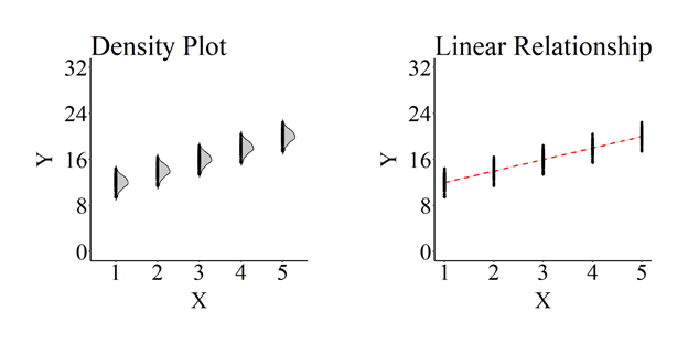
Furthermore, an OLS regression model was estimated where Y was regressed on X for the 1,000 cases. The estimates produced by the OLS regression model indicate that the slope coefficient was 2.000, the standard error of the association was .023, the p-value < .001, and the standardized slope coefficient was .937.
M<-lm(Y~X,data = df1) # Model of Y regressed on X

summary(M) # Summary of Results (estimate = b)

Call:
lm(formula = Y ~ X, data = df1)

Residuals:
          Min            1Q        Median            3Q           Max
-2.5823123488 -0.6183026704  0.0184348923  0.7294629685  2.4902740119

Coefficients:
                Estimate   Std. Error   t value               Pr(>|t|)
(Intercept) 9.9949045000 0.0778204590 128.43543 < 0.000000000000000222 ***
X           2.0000000000 0.0234637512  85.23786 < 0.000000000000000222 ***
---
Signif. codes:  0 ‘***’ 0.001 ‘**’ 0.01 ‘*’ 0.05 ‘.’ 0.1 ‘ ’ 1

Residual standard error: 1.04933086 on 998 degrees of freedom
Multiple R-squared:  0.879227831,	Adjusted R-squared:  0.879106816
F-statistic: 7265.49319 on 1 and 998 DF,  p-value: < 0.0000000000000002220446

lm.beta(M) # Standardized Coefficient for Association

Call:
lm(formula = Y ~ X, data = df1)

Standardized Coefficients::
   (Intercept)              X
0.000000000000 0.937671493949
Violating the Homoscedasticity Assumption
Now that we have simulated a homoscedastic relationship and estimated the coefficients using an OLS regression model, we must violate the model assumptions by specifying a heteroscedastic relationship between the variables. The relationship between X and Y can be simulated as heteroscedastic by simply replicating the specification but varying the standard deviation value for the five distinct Y constructs (reminder: Y1 is to X = 1 as Y5 is to X = 5). Varying the standard deviation specification will ensure that the distribution of scores on the dependent variable is not consistent across scores of the independent variable. For illustrative purposes, three simulations with distinct specification patterns for the standard deviation were constructed. These patterns of specifying the standard deviations were: (1) an inconsistent specification, (2) an expanding specification, and (3) a tightening specification.
The inconsistent specification – as alluded to by the name – were just values selected by myself when specifying the standard deviation of the five distinct Y constructs. I, with no reason in mind, selected the values .2, 3, 1.4, 4, .4.[ii] After specifying the five distinct Y constructs, the remaining steps of the specification were repeated, the graphs were produced, and an OLS regression model was estimated.
n<-200 # N-Size
set.seed(12) # Seed
X<-rep(c(1:5), each = n) # Repeat Each Value 200 times

set.seed(15)
Y1<-2+rnorm(n,10,.2) # Y1 Specification
set.seed(15)
Y2<-4+rnorm(n,10,3) # Y2 Specification
set.seed(15)
Y3<-6+rnorm(n,10,1.4) # Y3 Specification
set.seed(15)
Y4<-8+rnorm(n,10,4) # Y4 Specification
set.seed(15)
Y5<-10+rnorm(n,10,.4) # Y5 Specification

Y<-rep(NA, each = 1000) # Empty Vector for Y with 1000 cells

df1<-data.frame(X,Y) # Dataframe containing X and Y (Empty Vector)
df1$Y[df1$X==1]<-Y1 # When X = 1, Y = Y1
df1$Y[df1$X==2]<-Y2 # When X = 2, Y = Y2
df1$Y[df1$X==3]<-Y3 # When X = 3, Y = Y3
df1$Y[df1$X==4]<-Y4 # When X = 4, Y = Y4
df1$Y[df1$X==5]<-Y5 # When X = 5, Y = Y5
As demonstrated in the plot below, and consistent with our specifications, the distribution of scores on Y across values of X is not consistent. Specifically, the distribution of scores on Y when X equals 1, 3, or 5 is substantively tighter than the distribution of scores on Y when X equals 2 or 4. The differences between the distributions for Y at different scores on X means that we properly specified a heteroscedastic association. The density plot provides the perfect visual illustration of heteroscedasticity. Excluding the visual differences in the plotted values, the slope of the regression line for the heteroscedastic relationship appears to be – and is almost – identical to the slope of the regression for the homoscedastic specification. The key difference between the linear relationship plots is the estimated standard error represented by the gray area.
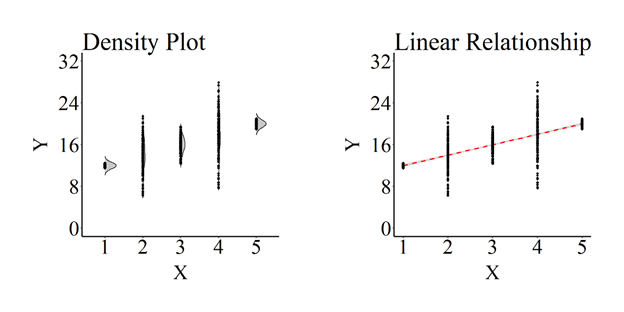
Although visually similar, the estimated standard error of the association between X and Y almost doubles to .054 (Non-violated SE = .023) and the standardized slope coefficient is reduced to .757 (Non-violated β = .937).
M<-lm(Y~X,data = df1)

summary(M)

Call:
lm(formula = Y ~ X, data = df1)

Residuals:
          Min            1Q        Median            3Q           Max
-10.339746125  -0.597435168   0.015822992   0.652115189   9.950599318

Coefficients:
                Estimate   Std. Error  t value               Pr(>|t|)
(Intercept) 9.9929682100 0.1813742803 55.09584 < 0.000000000000000222 ***
X           1.9992866300 0.0546864031 36.55912 < 0.000000000000000222 ***
---
Signif. codes:  0 ‘***’ 0.001 ‘**’ 0.01 ‘*’ 0.05 ‘.’ 0.1 ‘ ’ 1

Residual standard error: 2.4456503 on 998 degrees of freedom
Multiple R-squared:  0.572512111,	Adjusted R-squared:  0.572083767
F-statistic: 1336.56906 on 1 and 998 DF,  p-value: < 0.0000000000000002220446

lm.beta(M)

Call:
lm(formula = Y ~ X, data = df1)

Standardized Coefficients::
   (Intercept)              X
0.000000000000 0.756645300717
The exact same pattern of results can be observed when the distribution of scores on Y expands as values on X increase and when the distribution of scores on Y tightens as values on X increase.
Expanding Distribution
The specification for Y possessing an expanding distribution across values of X is:
n<-200 # N-Size
set.seed(12) # Seed
X<-rep(c(1:5), each = n) # Repeat Each Value 200 times

set.seed(15)
Y1<-2+rnorm(n,10,1) # Y1 Specification
set.seed(15)
Y2<-4+rnorm(n,10,1.7) # Y2 Specification
set.seed(15)
Y3<-6+rnorm(n,10,2.4) # Y3 Specification
set.seed(15)
Y4<-8+rnorm(n,10,3.1) # Y4 Specification
set.seed(15)
Y5<-10+rnorm(n,10,3.8) # Y5 Specification

Y<-rep(NA, each = 1000) # Empty Vector for Y with 1000 cells

df1<-data.frame(X,Y) # Dataframe containing X and Y (Empty Vector)
df1$Y[df1$X==1]<-Y1 # When X = 1, Y = Y1
df1$Y[df1$X==2]<-Y2 # When X = 2, Y = Y2
df1$Y[df1$X==3]<-Y3 # When X = 3, Y = Y3
df1$Y[df1$X==4]<-Y4 # When X = 4, Y = Y4
df1$Y[df1$X==5]<-Y5 # When X = 5, Y = Y5
The plotted association is:
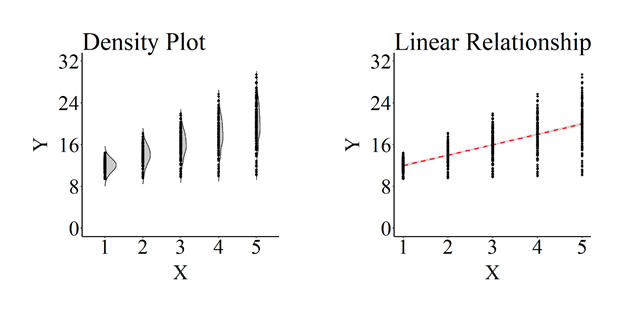
Below are the coefficients estimated from an OLS regression model.
M<-lm(Y~X,data = df1)

summary(M)

Call:
lm(formula = Y ~ X, data = df1)

Residuals:
         Min           1Q       Median           3Q          Max
-9.812786926 -1.359686355  0.030912321  1.529959707  9.463041245

Coefficients:
                Estimate   Std. Error  t value               Pr(>|t|)
(Intercept) 9.9984713500 0.2020336623 49.48914 < 0.000000000000000222 ***
X           1.9964331500 0.0609154412 32.77384 < 0.000000000000000222 ***
---
Signif. codes:  0 ‘***’ 0.001 ‘**’ 0.01 ‘*’ 0.05 ‘.’ 0.1 ‘ ’ 1

Residual standard error: 2.72422135 on 998 degrees of freedom
Multiple R-squared:  0.518368786,	Adjusted R-squared:  0.517886189
F-statistic: 1074.12483 on 1 and 998 DF,  p-value: < 0.0000000000000002220446

lm.beta(M)

Call:
lm(formula = Y ~ X, data = df1)

Standardized Coefficients::
   (Intercept)              X
0.000000000000 0.719978322972
Tightening Distribution
The specification for Y possessing an tightening distribution across values of X is:
n<-200 # N-Size
set.seed(12) # Seed
X<-rep(c(1:5), each = n) # Repeat Each Value 200 times

set.seed(15)
Y1<-2+rnorm(n,10,3.8) # Y1 Specification
set.seed(15)
Y2<-4+rnorm(n,10,3.1) # Y2 Specification
set.seed(15)
Y3<-6+rnorm(n,10,2.4) # Y3 Specification
set.seed(15)
Y4<-8+rnorm(n,10,1.7) # Y4 Specification
set.seed(15)
Y5<-10+rnorm(n,10,1) # Y5 Specification

Y<-rep(NA, each = 1000) # Empty Vector for Y with 1000 cells

df1<-data.frame(X,Y) # Dataframe containing X and Y (Empty Vector)
df1$Y[df1$X==1]<-Y1 # When X = 1, Y = Y1
df1$Y[df1$X==2]<-Y2 # When X = 2, Y = Y2
df1$Y[df1$X==3]<-Y3 # When X = 3, Y = Y3
df1$Y[df1$X==4]<-Y4 # When X = 4, Y = Y4
df1$Y[df1$X==5]<-Y5 # When X = 5, Y = Y5
The plotted association is:

Below are the coefficients estimated from an OLS regression model.
M<-lm(Y~X,data = df1)

> summary(M)

Call:
lm(formula = Y ~ X, data = df1)

Residuals:
         Min           1Q       Median           3Q          Max
-9.812786926 -1.359686355  0.030912321  1.529959707  9.463041245

Coefficients:
                Estimate   Std. Error  t value               Pr(>|t|)
(Intercept) 9.9770702501 0.2020336623 49.38321 < 0.000000000000000222 ***
X           2.0035668500 0.0609154412 32.89095 < 0.000000000000000222 ***
---
Signif. codes:  0 ‘***’ 0.001 ‘**’ 0.01 ‘*’ 0.05 ‘.’ 0.1 ‘ ’ 1

Residual standard error: 2.72422135 on 998 degrees of freedom
Multiple R-squared:  0.520149565,	Adjusted R-squared:  0.519668752
F-statistic: 1081.81472 on 1 and 998 DF,  p-value: < 0.0000000000000002220446

> lm.beta(M)

Call:
lm(formula = Y ~ X, data = df1)

Standardized Coefficients::
   (Intercept)              X
0.000000000000 0.721213951981
Distinct from other assumptions, violating the homoscedasticity assumption will not alter the regression line estimated in an OLS regression model. Standard errors, however, will be upwardly biased, while hypothesis tests and the standardized slope coefficients will be downwardly biased. The same holds true in multivariable models.
Violating the Homoscedasticity Assumption: Multivariable Models
The simulation code provided below relies on the simpler method of simulating homoscedastic and heteroscedastic associations.[iii] The simulation begins by specifying that C (representing “confounder”) is a random sample of 1,000 values ranging between 1 and 5 and X is equal to 1*C plus a random sample of 1,000 values ranging between 1 and 5. This specification ensures that C confounds the association between X and Y. The simulation is then specified to set scores on the dependent variable (Y) equal to 2*X plus 1*C plus 2* a normal distribution of values. The normal distribution of values is set to have a mean of 15 and a standard deviation of 1 for the homoscedastic specification, while the normal distribution of values is set to have a mean of 15 and a standard deviation equal to the square root of X*C raised to the 1.5 power for the heteroscedastic association. The results of violating the homoscedasticity assumption in a multivariable OLS regression model directly emulates the bivariate results reviewed above.
Multivariable Homoscedastic Association
The following R-code is used to specify a homoscedastic multivariable association.
n<-1000
set.seed(12)
C<-sample(c(1:5),size=n, replace = T)
set.seed(43)
X<-.1*C+2*sample(c(1:5),size=n, replace = T)
set.seed(29)
Y<-2*X+1*C+5*rnorm(n,15,1)
df1<-data.frame(X,Y,C)
To plot the bivariate association between X and Y, the Y-residuals were calculated. The y-axis on the density plot and linear relationship plot are the Y residuals.

Below are the coefficients estimated from an OLS regression model.
M<-lm(Y~X+C,data = df1)

summary(M)

Call:
lm(formula = Y ~ X + C, data = df1)

Residuals:
          Min            1Q        Median            3Q           Max
-16.069812664  -3.585479819  -0.038827947   3.816366395  15.775871868

Coefficients:
                 Estimate    Std. Error   t value               Pr(>|t|)
(Intercept) 75.5558677681  0.5565820207 135.74975 < 0.000000000000000222 ***
X            1.8937163747  0.0603399595  31.38412 < 0.000000000000000222 ***
C            0.9686775249  0.1190453249   8.13705  0.0000000000000011985 ***
---
Signif. codes:  0 ‘***’ 0.001 ‘**’ 0.01 ‘*’ 0.05 ‘.’ 0.1 ‘ ’ 1

Residual standard error: 5.35416372 on 997 degrees of freedom
Multiple R-squared:  0.512197284,	Adjusted R-squared:  0.511218743
F-statistic:  523.42953 on 2 and 997 DF,  p-value: < 0.0000000000000002220446

> lm.beta(M)

Call:
lm(formula = Y ~ X + C, data = df1)

Standardized Coefficients::
   (Intercept)              X              C
0.000000000000 0.694225418791 0.179993768445
Multivariable Heteroscedastic Association
The following R-code is used to specify a Heteroscedastic multivariable association.
n<-1000
set.seed(12)
C<-sample(c(1:5),size=n, replace = T)
set.seed(43)
X<-.1*C+2*sample(c(1:5),size=n, replace = T)
set.seed(29)
Y<-2*X+1*C+2*rnorm(n,15,sqrt((X*C)^1.5))
df1<-data.frame(X,Y,C)
To plot the bivariate association between X and Y, the Y-residuals were calculated. The y-axis on the density plot and linear relationship plot are the Y residuals.

Below are the coefficients estimated from an OLS regression model.
M<-lm(Y~X+C,data = df1)

summary(M)

Call:
lm(formula = Y ~ X + C, data = df1)

Residuals:
         Min           1Q       Median           3Q          Max
-94.82062676  -9.77572616  -0.25253024  10.81786931  91.49539700

Coefficients:
                Estimate   Std. Error  t value               Pr(>|t|)
(Intercept) 33.198290533  2.244998933 14.78766 < 0.000000000000000222 ***
X            1.497595236  0.243383975  6.15322        0.0000000010981 ***
C            0.614402524  0.480174741  1.27954                  0.201
---
Signif. codes:  0 ‘***’ 0.001 ‘**’ 0.01 ‘*’ 0.05 ‘.’ 0.1 ‘ ’ 1

Residual standard error: 21.5962632 on 997 degrees of freedom
Multiple R-squared:  0.0379854149,	Adjusted R-squared:  0.0360555963
F-statistic: 19.6834119 on 2 and 997 DF,  p-value: 0.00000000413100503

> lm.beta(M)

Call:
lm(formula = Y ~ X + C, data = df1)

Standardized Coefficients::
    (Intercept)               X               C
0.0000000000000 0.1911444894215 0.0397477905866
Conclusions
Violations of the homoscedasticity assumption do bias estimates produced by OLS regression models. The estimates influenced by violations of the homoscedasticity assumption are the standard error, t-value, p-value, and the standardized slope coefficients. Although the degree of bias can vary dependent upon the inconsistencies in the width of the Y distribution across scores on X, the direction of the bias will remain consistent across all heteroscedastic associations. Specifically, the standard error and the p-value will be upwardly biased, while the t-value and the standardized slope coefficients will be downwardly biased.[iv] This means that estimating a hypothesis test on a heteroscedastic association will increase the likelihood of committing type 2 errors (failing to reject the null hypothesis when we should’ve rejected the null hypothesis) but not increase our likelihood of committing type 1 errors (rejecting the null hypothesis when we should’ve failed to reject the null hypothesis). In conclusion, although we should make efforts to reduce our likelihood of violating model assumptions, violating the homoscedasticity assumption can only serve to reduce the likelihood of rejecting the null hypothesis.
[i] Although more complicated, simulating the relationship in this manner provides the ability to alter the structure of the heteroscedasticity in an inconsistent manner, which is key to one of the subsequent examples.
[ii] Now looking back upon it, the values I randomly chose do create a pattern…
[iii] The specification process used for the bivariate associations cannot be easily translated to multivariable models.
[iv] The slope coefficient estimated when homoscedasticity is violated could slightly vary but not enough to fall outside of the confidence intervals of the slope coefficient when homoscedasticity is satisfied
License: Creative Commons Attribution 4.0 International (CC By 4.0)
