Satisfying the assumption of linearity in an Ordinary Least Squares (OLS) regression model is vital to the development of unbiased slope coefficients, standardized coefficients, standard errors, and the model R2. Simply put, if a non-linear relationship exists, the estimates produced from specifying a linear association between two variables will be biased. But how biased will the slope coefficients, standardized coefficients, standard errors, and model R2 be when we violate the linearity assumption in OLS regression model? Moreover, what would violating the linearity assumption do to our interpretation of an association between two variables?
Let’s start with a basic review of the linearity assumption. The linearity assumption is the belief that the expected value of a dependent variable will change at a constant rate across values of an independent variable (i.e., a linear function). To provide an example of the linearity assumption, if we increase the independent variable by 1-point and observe a 1-point increase in the dependent variable, we would assume that any subsequent 1-point increase in the independent variable would result in a 1-point increase in the dependent variable. Although mathematically logical, non-linear associations often exist between variables. A non-linear association is simply a relationship where the direction and rate of change in the dependent variable will differ as we increase the score on the independent variable. Considering the example above, if the relationship is non-linear we would not assume that any subsequent 1-point increase in the independent variable would result in a 1-point increase in the dependent variable.
Determining if an association is linear or non-linear is important as it guides how we specify OLS regression models. For a linear association (the most common assumption) we would regress the dependent variable on the independent variable, and for a non-linear association with a single curve we would regress the dependent variable on the independent variable and the independent variable squared. The differences between the specifications simply inform the model that we either expect a linear association or expect a threshold (i.e., curve) to exist in the association of interest. If our expectations and specifications do not match the observed data, we would violate our assumptions in the estimated model. More often than not, we assume that a linear association exists between the dependent variable and the independent variable because theory and prior research rarely guide us to the alternative. However, if the observed data violates this assumption (the linearity assumption), the results of our models could be biased.
To determine the degree of bias that exists after violating the linearity assumption, we will conduct directed equation simulations. Simulations are a common analytical technique used to explore how the coefficients produced by statistical models deviate from reality (the simulated relationship) when certain assumptions are violated. The current analysis focuses on violations of the linearity assumption.
Satisfying the Linearity Assumption: Linear Association
We will first begin by simulating a linear relationship between a dependent variable (identified as Y in the code) and an independent variable (identified as X in the code). All of the examples reviewed from herein are based on 100 cases (identified as n in the code). The dependent variable (X) is specified as a normally distributed construct with a mean of 5 and a standard deviation of 1. If we did not specify X as a normally distributed construct we would run the risk of violating other assumptions and create an ambiguous examination of the degree of bias that exists after violating the linearity assumption. After simulating X, we specify that Y is equal to .25×X plus .025×normally distributed error. In this example, .25 is the true slope coefficient for the relationship between X and Y, where a 1-point increase in X corresponds to a .25 increase in Y. Including normally distributed error ensures we don’t perfectly predict the dependent variable when estimating the regression model. Importantly, the set.seed portion of the code ensures that the random variables are equal each time we run a simulation.
> n<-100 # Sample size
> set.seed(1001) # Seed
> X<-rnorm(n,5,1) # Specification of the independent variable
> set.seed(32) # Seed
> Y<-.25*X+.025*rnorm(n,5,1) # Specification of the dependent variable
Now that we have our data, let’s estimate an OLS regression model. Following the R-code for estimating a regression model, we regress Y on X. The results suggest that the slope coefficient for the association is .250, the standard error is .002, and the standardized coefficient is .997. This is exactly what we would expect to find given the specification of the data. In addition to just estimating the model, let’s plot this relationship using ggplot2. Ggplot2 is the best package ever. As demonstrated, the specification of the relationship between X and Y in our first simulated dataset is perfectly linear (a 1-point increase in X corresponds to a .25-point increase in Y).
> M<-lm(Y~X) # Estimating regression model (Linear relationship between X and Y assumed)
>
> # Results
> summary(M) # Summary of model results

Call:
lm(formula = Y ~ X)

Residuals:
           Min             1Q         Median             3Q            Max
-0.06579416011 -0.01478787853  0.00240413934  0.01523569058  0.04045840087

Coefficients:
                 Estimate    Std. Error   t value               Pr(>|t|)
(Intercept) 0.12328940395 0.00975526777  12.63824 < 0.000000000000000222 ***
X           0.25002056505 0.00190264638 131.40674 < 0.000000000000000222 ***
---
Signif. codes:  0 ‘***’ 0.001 ‘**’ 0.01 ‘*’ 0.05 ‘.’ 0.1 ‘ ’ 1

Residual standard error: 0.0216664405 on 98 degrees of freedom
Multiple R-squared:  0.994356702,	Adjusted R-squared:  0.994299117
F-statistic: 17267.7323 on 1 and 98 DF,  p-value: < 0.0000000000000002220446

>
> library(lm.beta)
> lm.beta(M) # Standardized coefficients

Call:
lm(formula = Y ~ X)

Standardized Coefficients::
   (Intercept)              X
0.000000000000 0.997174358939

Violating the Linearity Assumption
We are presented with a unique challenge when simulating a curvilinear association between our dependent and independent variables. Similar to the preceding example, the independent variable (X) is specified as a normally distributed variable with a mean of 5 and a standard deviation of 1. To simulate a curvilinear association, however, we need to include another specification of X that is X2 (labeled as X2 in the model). We can create X2 by multiplying X by X or specifying X^2. For simplicity we rely on the former. Next, Y is defined to have a positive .25 slope coefficient with X, a negative .025 slope coefficient with X2, and a .025 slope coefficient with the normally distributed error. Again, the normally distributed error only serves to ensure that our model does not perfectly predict Y.
> set.seed(1001)
> X<-rnorm(n,5,1) # Specification of the independent variable
> X2<-X*X # Specification of the independent variable squared
> set.seed(32)
> Y<-(.25*X)-.025*X2+.025*rnorm(n,5,1) # Specification of the dependent variable
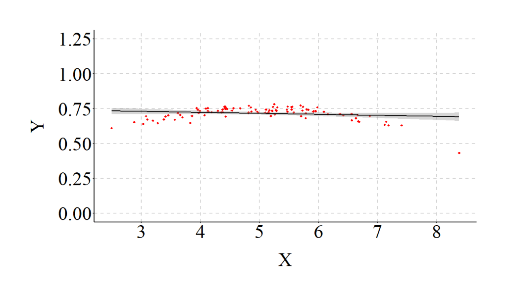
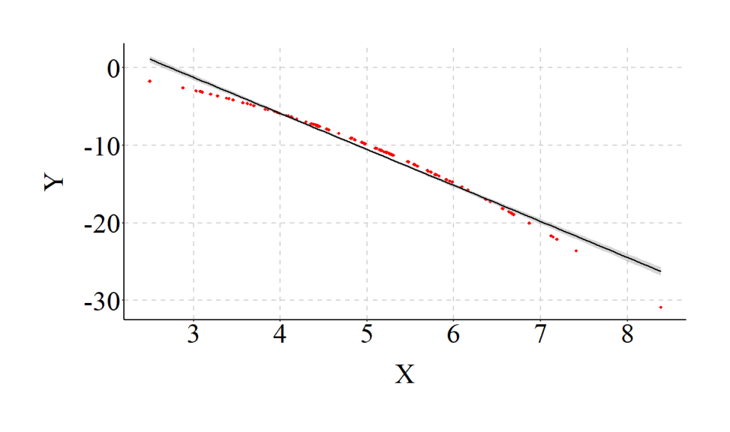
After simulating a curvilinear association in the data, we estimate a regression model After simulating a curvilinear association in the data, we estimate a regression model that assumes a linear association between Y and X (we are knowingly violating the linearity assumption). The findings of the misspecified model suggest that a 1-point increase in X is associated with a .007 decrease in Y (SE = .004; β = -.173). Consistent with the misspecification, the estimated slope coefficient deviates from the specified slope coefficients between X and Y, and X2 and Y. Additionally, the R2 value suggests that the linear specification of the association only explains .02 percent of the variation in Y, which is a substantial departure from reality.
> # Misspecified model (Linear relationship between X and Y assumed)
> Mis<-lm(Y~X)
>
> # Results
> summary(Mis)

Call:
lm(formula = Y ~ X)

Residuals:
          Min            1Q        Median            3Q           Max
-0.2597571656 -0.0206712212  0.0113012471  0.0283234287  0.0682318921

Coefficients:
                  Estimate     Std. Error  t value             Pr(>|t|)
(Intercept)  0.75134794607  0.02089728531 35.95433 < 0.0000000000000002 ***
X           -0.00707614052  0.00407576144 -1.73615              0.08568 .
---
Signif. codes:  0 ‘***’ 0.001 ‘**’ 0.01 ‘*’ 0.05 ‘.’ 0.1 ‘ ’ 1

Residual standard error: 0.0464128509 on 98 degrees of freedom
Multiple R-squared:  0.0298395903,	Adjusted R-squared:  0.0199399943
F-statistic: 3.01422303 on 1 and 98 DF,  p-value: 0.0856797297

> lm.beta(Mis)

Call:
lm(formula = Y ~ X)

Standardized Coefficients::
    (Intercept)               X
 0.000000000000 -0.172741397271
Moreover, as demonstrated in the figure below, the specification of a linear relationship – for our curvilinear data – creates a relatively horizontal OLS regression line.
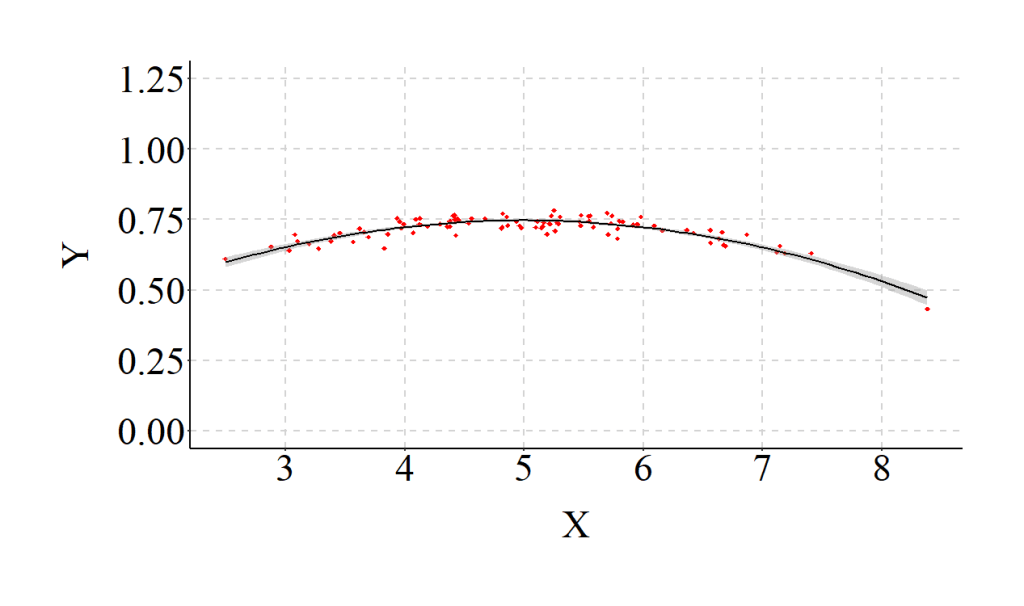
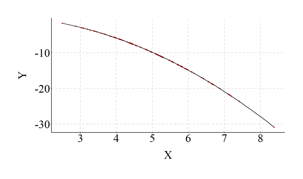
To make sure the example was completed correctly, however, we should estimate a model that properly specifies the relationship (i.e., the inclusion of X2 in the regression model) and compare the results. As expected, when we estimate the model assuming a curvilinear association we observe coefficients that match our specification. Additionally, the R2 jumps from .02 to .79, indicating that the explanatory power of our model substantively increases when the relationship is properly specified.
> # Properly Specified Model (Curvilinear relationship between X and Y assumed)
> PS<-lm(Y~X+I(X^2))
>
> # Results
> summary(PS)

Call:
lm(formula = Y ~ X + I(X^2))

Residuals:
           Min             1Q         Median             3Q            Max
-0.06629449249 -0.01476256564  0.00216027121  0.01361241435  0.03760637947

Coefficients:
                  Estimate     Std. Error   t value               Pr(>|t|)
(Intercept)  0.15397661671  0.03328538416   4.62595             0.00001153 ***
X            0.23745870851  0.01316497818  18.03715 < 0.000000000000000222 ***
I(X^2)      -0.02377848916  0.00126670865 -18.77187 < 0.000000000000000222 ***
---
Signif. codes:  0 ‘***’ 0.001 ‘**’ 0.01 ‘*’ 0.05 ‘.’ 0.1 ‘ ’ 1

Residual standard error: 0.0216741925 on 97 degrees of freedom
Multiple R-squared:  0.790589444,	Adjusted R-squared:  0.786271701
F-statistic: 183.102461 on 2 and 97 DF,  p-value: < 0.0000000000000002220446

> lm.beta(PS)

Call:
lm(formula = Y ~ X + I(X^2))

Standardized Coefficients::
   (Intercept)              X         I(X^2)
 0.00000000000  5.79679685375 -6.03292108222
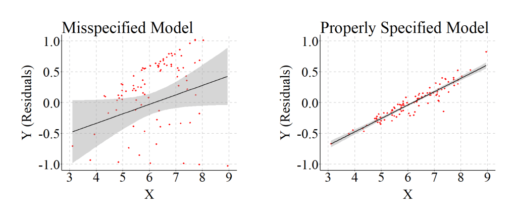
The differences between the estimates for the misspecified model and the properly specified model provide an illustration of how our interpretations can change when we violate the linearity assumption. The standardized coefficients from the misspecified model suggest that X has a negligible linear effect on Y. Nevertheless, this negligible linear effect does not represent reality. Our specification – reviewed above – dictates that X has a substantive and statistically significant curvilinear association with Y, where X has a positive influence on Y until the threshold, and then has a negative influence on Y.
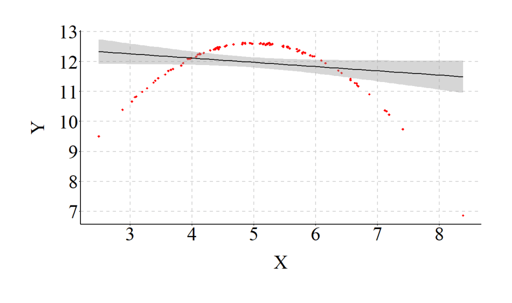
Taking this example to an extreme (specification in the code), we can see that the Taking this example to an extreme (specification in the code), we can see that the magnitude – or strength – of a linear regression line fit on curvilinear data is substantially weaker than reality (i.e., the specifications of the data). Of particular importance is the observation that X has minimal influence on Y in the misspecified model.
> set.seed(1001)
> X<-rnorm(n,5,1)
> X2<-X*X
> set.seed(32)
> Y<-5.00*X-.50*X2+.025*rnorm(n,5,1)
> # Misspecified model (Linear relationship between X and Y assumed)
> Mis<-lm(Y~X)
>
> summary(Mis)

Call:
lm(formula = Y ~ X)

Residuals:
         Min           1Q       Median           3Q          Max
-4.631367315 -0.337941262  0.360400075  0.582827465  0.688120764

Coefficients:
                 Estimate    Std. Error  t value             Pr(>|t|)
(Intercept) 12.6844602464  0.3882829355 32.66809 < 0.0000000000000002 ***
X           -0.1419135464  0.0757298661 -1.87394             0.063917 .
---
Signif. codes:  0 ‘***’ 0.001 ‘**’ 0.01 ‘*’ 0.05 ‘.’ 0.1 ‘ ’ 1

Residual standard error: 0.862376032 on 98 degrees of freedom
Multiple R-squared:  0.0345937282,	Adjusted R-squared:  0.0247426438
F-statistic: 3.51166702 on 1 and 98 DF,  p-value: 0.0639172523

> lm.beta(Mis)

Call:
lm(formula = Y ~ X)

Standardized Coefficients::
    (Intercept)               X
 0.000000000000 -0.185993892912
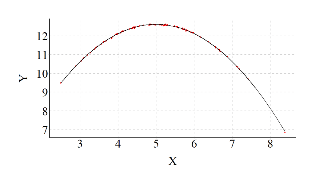
However, when we correctly assume the relationship is curvilinear and properly specify our model, the results align with reality.
> # Properly Specified Model (Curvilinear relationship between X and Y assumed)
> PS<-lm(Y~X+I(X^2))
>
> summary(PS)

Call:
lm(formula = Y ~ X + I(X^2))

Residuals:
           Min             1Q         Median             3Q            Max
-0.06629449249 -0.01476256564  0.00216027121  0.01361241435  0.03760637947

Coefficients:
                  Estimate     Std. Error    t value               Pr(>|t|)
(Intercept)  0.15397661671  0.03328538416    4.62595             0.00001153 ***
X            4.98745870851  0.01316497818  378.84291 < 0.000000000000000222 ***
I(X^2)      -0.49877848916  0.00126670865 -393.75944 < 0.000000000000000222 ***
---
Signif. codes:  0 ‘***’ 0.001 ‘**’ 0.01 ‘*’ 0.05 ‘.’ 0.1 ‘ ’ 1

Residual standard error: 0.0216741925 on 97 degrees of freedom
Multiple R-squared:  0.999396401,	Adjusted R-squared:  0.999383956
F-statistic: 80302.9033 on 2 and 97 DF,  p-value: < 0.0000000000000002220446

> lm.beta(PS)

Call:
lm(formula = Y ~ X + I(X^2))

Standardized Coefficients::
   (Intercept)              X         I(X^2)
 0.00000000000  6.53663363645 -6.79400644477
Exceptions
There are conditions where the shape of the association is curvilinear, but the misspecification of the relationship as linear only results in negligible reductions in There are conditions where the shape of the association is curvilinear, but the misspecification of the relationship as linear only results in negligible reductions in the variation explained by the model. The example below provides an illustration of this situation. The relationship is primarily negative and it is quite difficult to visually evaluate where the curve occurs. Although only negligible differences exist in the variation explained by the dependent variable, the unstandardized coefficient and standard error is considerably different than the specification.
> set.seed(1001)
> X<-rnorm(n,5,1)
> X2<-X*X
> set.seed(32)
> Y<-.50*X-.50*X2+.025*rnorm(n,5,1)
> # Misspecified model (Linear relationship between X and Y assumed)
> Mis<-lm(Y~X)
>
> summary(Mis)

Call:
lm(formula = Y ~ X)

Residuals:
         Min           1Q       Median           3Q          Max
-4.631367315 -0.337941262  0.360400075  0.582827465  0.688120764

Coefficients:
                 Estimate    Std. Error   t value               Pr(>|t|)
(Intercept) 12.6844602464  0.3882829355  32.66809 < 0.000000000000000222 ***
X           -4.6419135464  0.0757298661 -61.29568 < 0.000000000000000222 ***
---
Signif. codes:  0 ‘***’ 0.001 ‘**’ 0.01 ‘*’ 0.05 ‘.’ 0.1 ‘ ’ 1

Residual standard error: 0.862376032 on 98 degrees of freedom
Multiple R-squared:  0.974579526,	Adjusted R-squared:  0.974320134
F-statistic: 3757.16024 on 1 and 98 DF,  p-value: < 0.0000000000000002220446

> lm.beta(Mis)

Call:
lm(formula = Y ~ X)

Standardized Coefficients::
   (Intercept)              X
 0.00000000000 -0.98720794474
The results from a model assuming a curvilinear relationship between X and Y are presented below.
> # Properly Specified Model (Curvilinear relationship between X and Y assumed)
> PS<-lm(Y~X+I(X^2))
>
> summary(PS)

Call:
lm(formula = Y ~ X + I(X^2))

Residuals:
           Min             1Q         Median             3Q            Max
-0.06629449249 -0.01476256564  0.00216027121  0.01361241435  0.03760637947

Coefficients:
                  Estimate     Std. Error    t value               Pr(>|t|)
(Intercept)  0.15397661671  0.03328538416    4.62595             0.00001153 ***
X            0.48745870851  0.01316497818   37.02693 < 0.000000000000000222 ***
I(X^2)      -0.49877848916  0.00126670865 -393.75944 < 0.000000000000000222 ***
---
Signif. codes:  0 ‘***’ 0.001 ‘**’ 0.01 ‘*’ 0.05 ‘.’ 0.1 ‘ ’ 1

Residual standard error: 0.0216741925 on 97 degrees of freedom
Multiple R-squared:  0.999984106,	Adjusted R-squared:  0.999983779
F-statistic: 3051497.63 on 2 and 97 DF,  p-value: < 0.0000000000000002220446

> lm.beta(PS)

Call:
lm(formula = Y ~ X + I(X^2))

Standardized Coefficients::
    (Intercept)               X          I(X^2)
 0.000000000000  0.103669123728 -1.102459685779
Implications
Considering all of the examples reviewed thus far, it appears that the magnitude of the curve for the association determines the degree to which the misspecification of a linear relationship influences the slope coefficient, standard error, standardized effect and R2 value. Considering the potential effects, we should test if the association between the dependent variable and the independent variable of interest is linear or curvilinear before estimating our OLS regression models. This added step could help ensure that we don’t misspecify our model.
The Linearity Assumption in Multivariable Models
In and of itself, it is relatively easy to test and address the misspecification of a linear association between two variables. Misspecification of linear associations, however, become substantially more difficult to test and address in multivariable models. When dealing with a large number of covariates, conducting bivariate tests of the structure of the association between each covariate and the dependent variable could take large amount of time. Moreover, shared variation between constructs could invalidate the classifications determined by bivariate tests. This is all to say that we have an increased likelihood of misspefiying our model by assuming linear relationships. Though, why does it matter?
It matters because when we misspecify the structure of the association between a covariate and the dependent variable, the findings associated with the relationship of interest can be altered. The direction and magnitude of the bias introduced into the relationship, however, depends on the shape (i.e., standard bell curve or inverted bell curve) of the curvilinear association between the covariate and the dependent variable. To illustrate, let’s go back to the drawing board (or the simulation code).
Diminishing and Amplifying the Magnitude of the Relationship of Interest
Again, we will start off by simulating our data. This time, however, we will call our first variable C – for confounder – which is a normally distributed variable with a mean of 5 and a standard deviation of 1. Similar to the previous examples, we also multiple C by C to create our C2 term. For the purpose of this example, we want a linear association between our confounding variable (C) and our independent variable (X). As such, C2 is not included when simulating the data for X. The slope of the association between C and X is specified as .25, where a 1-point increase in C corresponds to a .25-point increase in X. Importantly, to ensure that the confounder does not completely nullify the association between X and Y, we specify that a large proportion of X is normally distributed and not influenced by C.
To simulate the dependent variable (Y), we now designate a linear relationship between X and Y, where a 1-point increase in X is associated with a .25 increase in Y. In addition to specifying a linear relationship between X and Y, we inform the computer that the confounder (or C) has a curvilinear effect on Y (Y = -4.0*C + .50*C2). Again, to ensure we don’t estimate a perfectly specified model, we include some normally distributed error in the simulation of Y.
> set.seed(1001)
> C<-rnorm(n,5,1)
> C2<-C*C
> set.seed(884680)
> X<-.25*C+1*rnorm(n,5,1)
> set.seed(32)
> Y<-(.25*X)+4.00*C+(-.50*C2)+.025*rnorm(n,5,1)
To compare the slope coefficients for the association between X and Y, we estimate one model assuming a linear association between C and Y (the misspecified model) and one model assuming a curvilinear association between C and Y (the properly specified model). For the misspecified model, the slope coefficient for Y on X is closer to zero (b = .173) than reality (b = .250). When compared to the properly specified model, the standard error also appears to be quite large (Misspecified SE = .084) and the magnitude of the standardized effects is reduced (Misspecified β = .127). In this example, the magnitude of the association between X and Y was attenuated when we assumed that a linear relationship existed between C and Y.
> # Misspecified model (Linear relationship between C and Y assumed)
> Mis<-lm(Y~X+C)
>
> summary(Mis)

Call:
lm(formula = Y ~ X + C)

Residuals:
         Min           1Q       Median           3Q          Max
-4.624276409 -0.351528084  0.323115155  0.565400618  0.797768249

Coefficients:
                 Estimate    Std. Error   t value             Pr(>|t|)
(Intercept) 13.0397899244  0.5461585065  23.87547 < 0.0000000000000002 ***
X            0.1726791657  0.0835168910   2.06760             0.041341 *
C           -1.1173989631  0.0802778032 -13.91915 < 0.0000000000000002 ***
---
Signif. codes:  0 ‘***’ 0.001 ‘**’ 0.01 ‘*’ 0.05 ‘.’ 0.1 ‘ ’ 1

Residual standard error: 0.863005351 on 97 degrees of freedom
Multiple R-squared:  0.674374746,	Adjusted R-squared:  0.667660824
F-statistic: 100.444222 on 2 and 97 DF,  p-value: < 0.0000000000000002220446

> lm.beta(Mis)

Call:
lm(formula = Y ~ X + C)

Standardized Coefficients::
    (Intercept)               X               C
 0.000000000000  0.126896684596 -0.854274488166
To reverse the effects, we will reverse the specification of the curvilinear association between C and Y (Y = -4.00*C + .50*C2). Every other specification remains the same.
> set.seed(1001)
> C<-rnorm(n,5,1)
> C2<-C*C
> set.seed(884680)
> X<-.25*C+1*rnorm(n,5,1)
> set.seed(32)
> Y<-(.25*X)+(-4.00*C)+(.50*C2)+.025*rnorm(n,5,1)
When the same comparison is conducted, it can be observed that the slope coefficient and the standard error for the association between X and Y is higher than reality (b = .321; SE = .084; p < .001).
> # Misspecified model (Linear relationship between C and Y assumed)
> Mis<-lm(Y~X+C)
>
> summary(Mis)

Call:
lm(formula = Y ~ X + C)

Residuals:
         Min           1Q       Median           3Q          Max
-0.834434950 -0.561855959 -0.340962810  0.329700840  4.565545886

Coefficients:
                  Estimate     Std. Error   t value               Pr(>|t|)
(Intercept) -12.7624272229   0.5492533751 -23.23596 < 0.000000000000000222 ***
X             0.3206221640   0.0839901488   3.81738             0.00023763 ***
C             1.1195639077   0.0807327064  13.86754 < 0.000000000000000222 ***
---
Signif. codes:  0 ‘***’ 0.001 ‘**’ 0.01 ‘*’ 0.05 ‘.’ 0.1 ‘ ’ 1

Residual standard error: 0.867895668 on 97 degrees of freedom
Multiple R-squared:  0.736643463,	Adjusted R-squared:  0.731213431
F-statistic: 135.660988 on 2 and 97 DF,  p-value: < 0.0000000000000002220446

> lm.beta(Mis)

Call:
lm(formula = Y ~ X + C)

Standardized Coefficients::
   (Intercept)              X              C
0.000000000000 0.210699184493 0.765415128876

As both examples illustrated, the findings associated with Y on X is altered by misspecifying the relationship between C and Y. More broadly, by misspecifying the structure of the associations between confounding variables and the dependent variable we can nullify or amplify the relationship between the dependent variable and the independent variable of interest. These misspecifications can result in an increased probability of type 1 (when the relationship is amplified) or type 2 error (when the relationship is nullified) and lead to conclusions not supported by reality. This highlights how cautious we should be when assuming linear relationships between our covariates and the dependent variable.
Conclusions
Overall, this demonstration is intended to illustrate how violating the linearity assumption in an OLS regression model effects the results of the model. Unlike other assumptions (which will be reviewed later), we can influence the slope coefficients, standard errors, and standardized effects in our model by accidentally violating the linearity assumption. To avoid the potential pitfalls associated with violating the linearity assumption, we should do our due diligence and examine if the dependent variable is linearly related to all of the constructs included in our models. If we suspect that the specification of a linear association between two constructs is not supported by the data, we can readily remedy this issue by specifying a curvilinear association or relying on alternative modeling strategies.
License: Creative Commons Attribution 4.0 International (CC By 4.0)
